TOPIC 6 · MAJOR ASSIGNMENT 3 · COMPONENT 01/ Probability / major assignment / analysis
01Mean, median, SD, range - then the empirical rule.
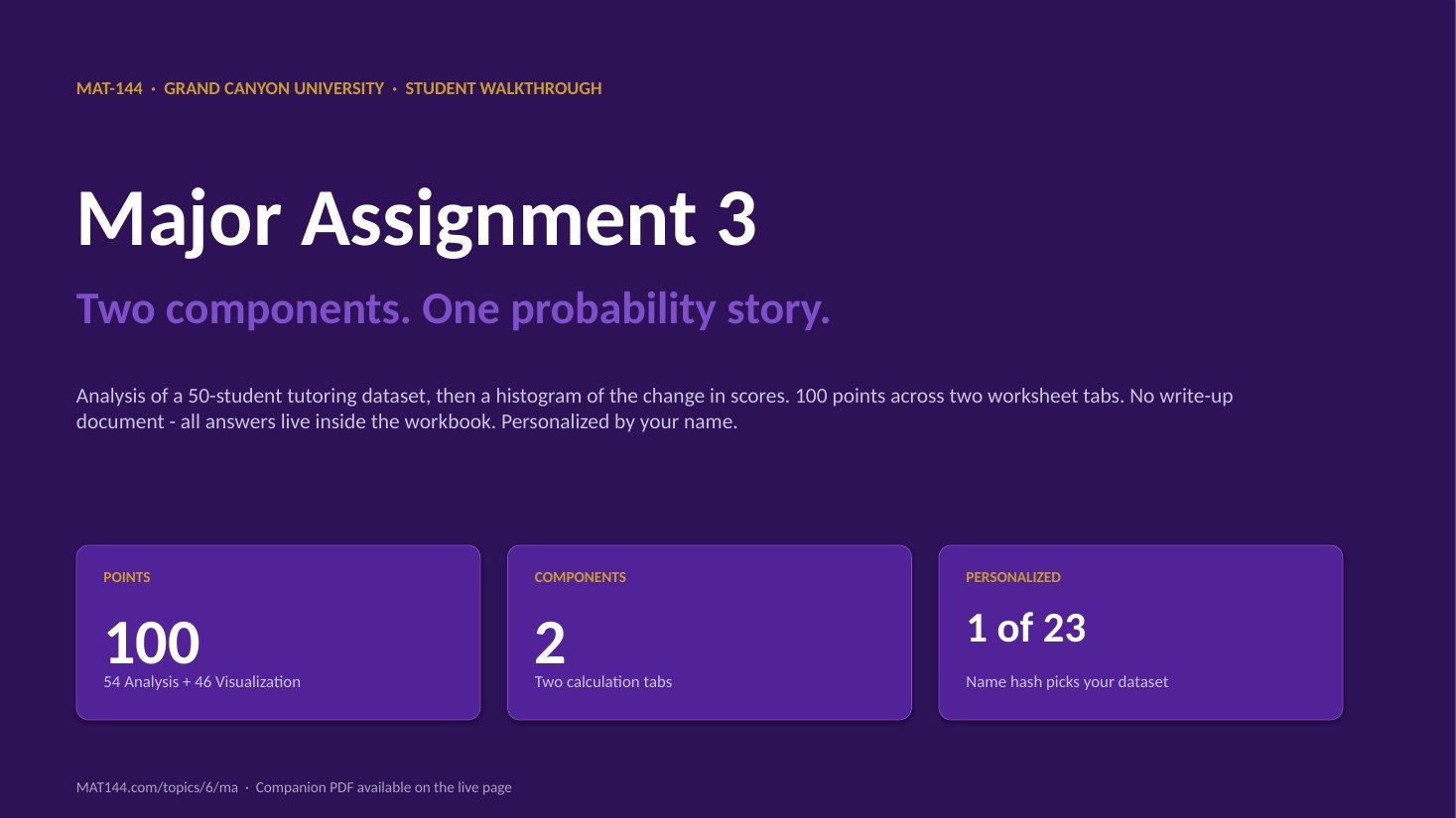
Enter your name, get a personalized 50-student tutoring study, compute the per-student score change, run descriptive stats across three columns, pull two percentiles, and apply the Empirical Rule to find the 68% interval on the change.
Major Assignment · 54 of 100 pts
50-student study
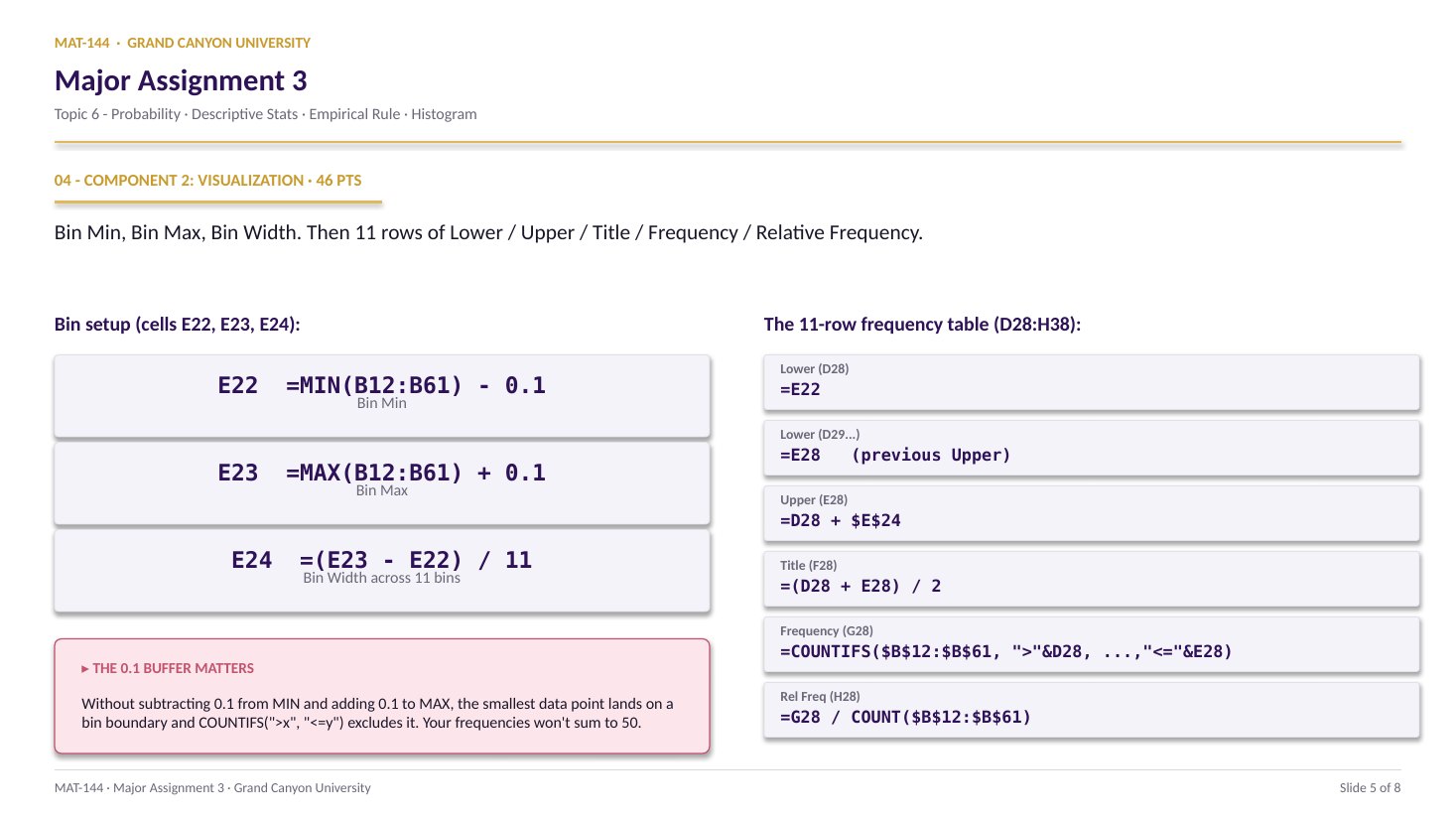
=AVERAGE() · =STDEV() · =PERCENTILE()
A 6-page MA3 Walkthrough PDF covers both components in the same hint depth as this page. Useful if you'd rather print, annotate on paper, or keep it open on a second screen while working in Excel.
Walkthrough video coming in a future recording. Until then, work from the slideshow above and the printable PDF.
SCRIBE.HOW · YOUTUBE
≡
Step-by-step walkthrough
Coming soon. Check back after the Scribe is recorded.
▸
Video walkthrough
Coming soon. Work from the slideshow and printable PDF until then.
MA3 C1 is Topic 5’s descriptive stats plus one probability handle. The five moves you already know from Topic 5 — mean, median, range, sample SD, and the Empirical Rule’s 68% interval — are exactly the columns MA3 C1 asks you to compute on the 50-row roster.
The attached video is Topic 5 Review Q5’s walkthrough of the Empirical Rule move (μ ± σ → 68%, μ ± 2σ → 95%, μ ± 3σ → 99.7%). That’s the same computation you’ll run in cells G36 / G37 for the lower / upper bounds of the 68% band.
If the arithmetic underneath still feels slippery, the Topic 5 Review Q3 walkthrough covers mean / median / mode on a single data set, and Topic 5 Review Q4 is the range move on its own. Both are the exact shape MA3 C1 asks for — only the data set differs.
Same walkthrough, three modes.Pick the one that lands for you today.
ORIENT
· the tab
Name first, then 50 differences, then the stats grid.
Cell B10 (your name) seeds the 23-column hash that picks your dataset. Then drag the difference formula down 50 rows, fill the 4x3 stats grid, look up two percentiles, compute the Empirical Rule bounds, and write the paragraph.
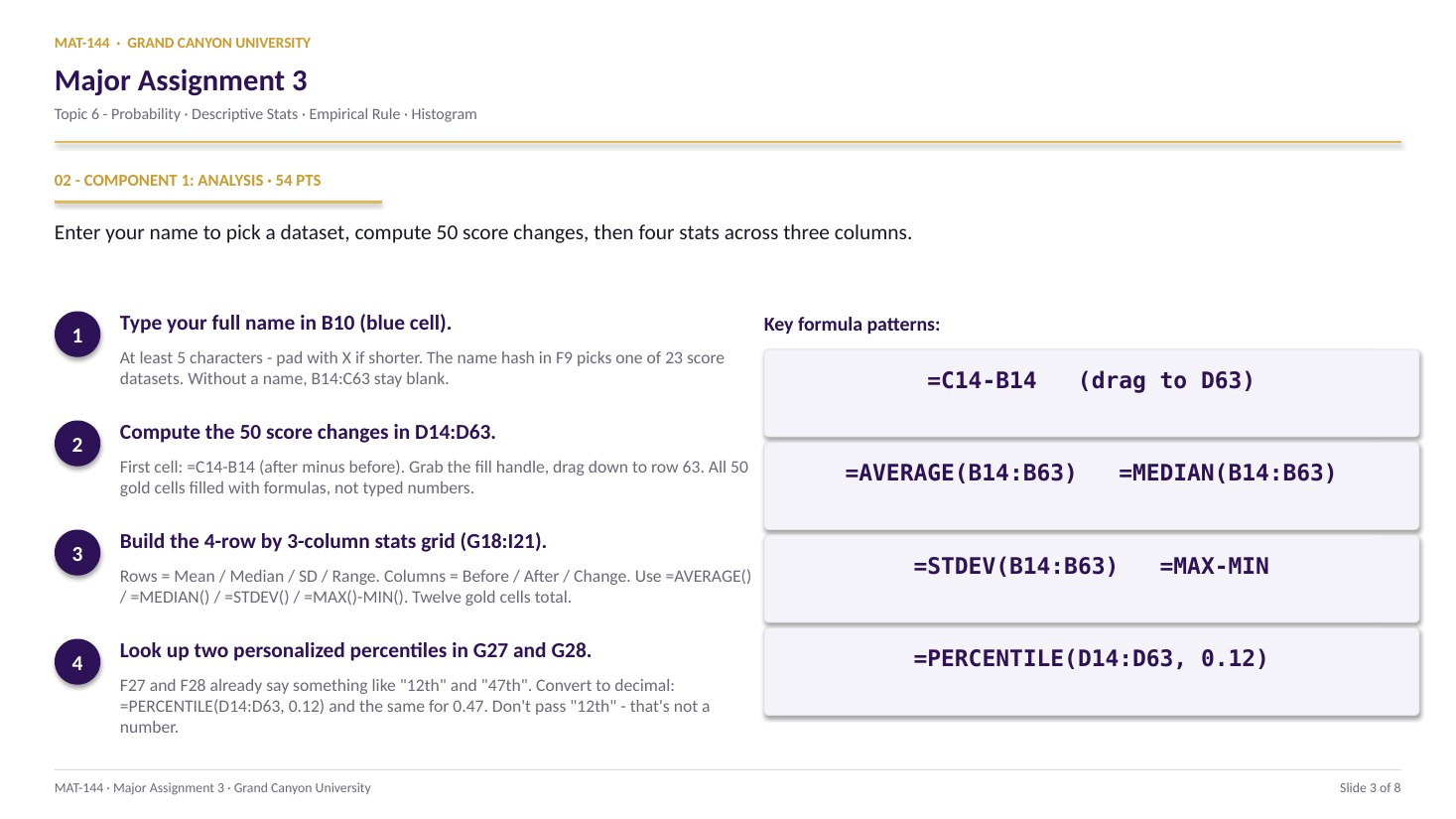
Your full name in B10 (blue cell, minimum 5 characters) is the only required text input. Until it is in, the 50-row score table is blank. Once it is, B14:B63 (Before) and C14:C63 (After) auto-populate from one of 23 personalized datasets. The hash result lives in F9 if you are curious which column you got.
§1 · Differences
D14:D63 - 50 rows of <em>after minus before.</em>
Gold column D needs =C14-B14 in the first cell, then drag down to D63. All 50 rows. Format as Number with 2 decimals.
Mean / Median / SD / Range as rows. Before / After / Change as columns. Twelve cells, twelve Excel functions, every one a cell range reference. Format Number with 2 decimals.
§3 · Percentiles
G27 + G28 from the <em>F27/F28 labels.</em>
F27 and F28 auto-generate labels like “12th” and “47th.” Convert by hand: 12th becomes 0.12. Formula: =PERCENTILE(D14:D63, 0.12).
§4 · Empirical Rule
G36 = H18 - H20 · G37 = H18 + H20.
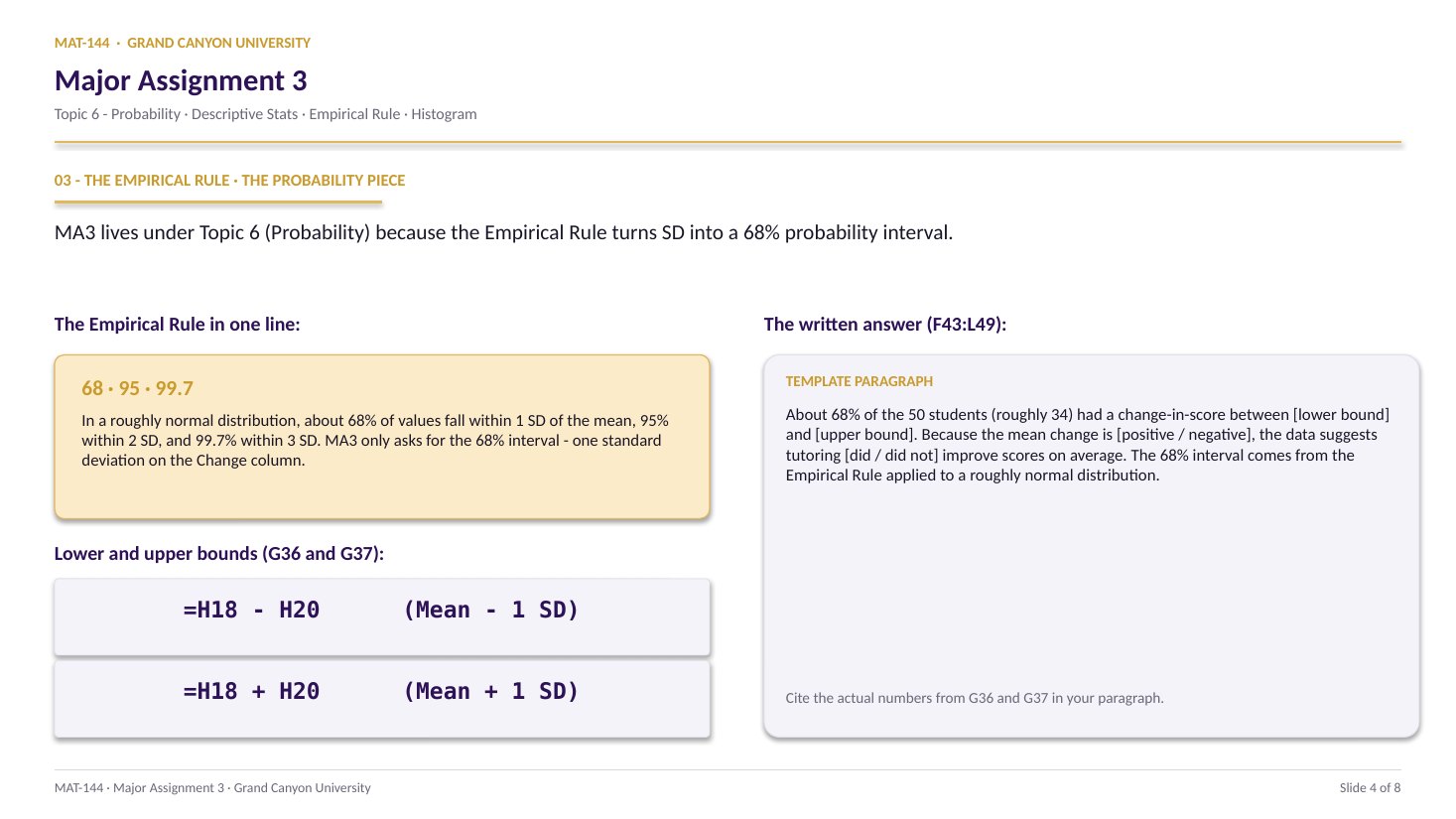
Mean of Change minus one SD of Change for the lower bound; plus one SD for the upper. The interval covers ~68% of the 50 students in a roughly normal distribution.
§5 · Written answer
F43:L49 - <em>cite your bounds.</em>
Two or three sentences. Quote G36 and G37. Say about 34 of the 50 students. Say whether tutoring helped. Generic statements lose points.
CONCEPTS · six things to know
The five moves you’ll make.
Name → differences → stats grid → percentiles → empirical rule. Click cells, never type numbers. Read your bounds, write the paragraph.
01
Name
B10 seeds your personalized dataset.
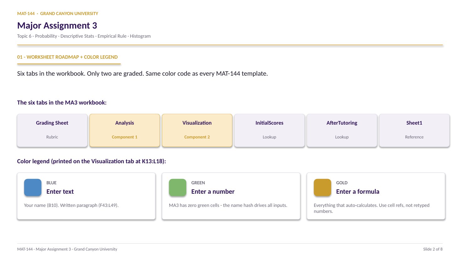
Cell B10 is the only required text input on the tab (besides the written paragraph in F43). Type your full name - at least 5 characters; pad with X if your name is shorter. The hash formula in F9 uses character codes to pick one of 23 personalized score columns from the InitialScores / AfterTutoring tabs.
Two students with different names get totally different score columns. Copying a classmate’s numbers fails the personalization audit - the grader sees the hash mismatch instantly. Type your real name, get your real dataset.
A
B
C
7
label
a
b
8
12
7
9
sum
=B8+C8
19
change B8→ C9 follows
02
Differences
=C14-B14, then drag to D63.
Gold cell D14 needs the formula =C14-B14 - after-tutoring minus before. Hover the bottom-right corner of D14 until you see the fill handle (small black cross), then drag down to D63. All 50 rows.
Self-check: click D63. The formula bar should read =C63-B63, not =C14-B14 and not a typed number. Relative references walk the column down for free. Format the entire range as Number with 2 decimal places.
D14 = =C14-B14
After-tutoring score minus before.
Drag the fill handle down through D63 - 50 rows.
03
·
B8+C8TEXT · LABEL
— PRESS = —
=
=B8+C815
Stats grid
Four rows, three columns - twelve functions.
The grid at G18:I21 needs four descriptive stats across three score columns. The pattern repeats row by row, column by column:
Row 18 - Mean:=AVERAGE(B14:B63) for Before, =AVERAGE(C14:C63) for After, =AVERAGE(D14:D63) for Change.
Row 19 - Median:=MEDIAN(B14:B63) and so on.
Row 20 - SD:=STDEV(B14:B63) and so on.
Row 21 - Range:=MAX(B14:B63) - MIN(B14:B63) and so on.
Format every cell as Number with 2 decimals. The Change column (column I in the grid, really H18-H21 in the worksheet) is the one Component 2 and the Empirical Rule both lean on.
04
Percentile
“12th” → 0.12, not the text.
Cells F27 and F28 auto-fill with percentile labels like “12th” and “47th.” =PERCENTILE() needs the decimal form, not the text. Convert by hand: “12th” means 0.12. “47th” means 0.47.
If you feed it the text string “12th” the function returns #VALUE! or #NUM!. Format the result as Number with 2 decimals.
=PERCENTILE(D14:D63, 0.12)
Range first, decimal percentile second.
Convert “12th” in F27 to 0.12 by hand.
05
Empirical Rule
Mean ± one SD covers ~68% of the data.
For a roughly normal distribution, ~68% of values fall within one standard deviation of the mean. The Change column has 50 values; 68% of 50 is 34. So the interval [mean - SD, mean + SD] should hold about 34 of your 50 students.
Cell G36 (Lower Bound): =H18 - H20 - mean of Change minus SD of Change. Cell G37 (Upper Bound): =H18 + H20. Format Number with 2 decimals.
The written answer in F43 needs both numbers cited literally - something like “About 34 of the 50 students saw their scores change by between [G36 value] and [G37 value], which suggests tutoring did improve scores on average.”
Cell by cell
=(E21+E22+E23+…+E28)/8
⟶
Range, scales freely
=AVERAGE(E21:E28)
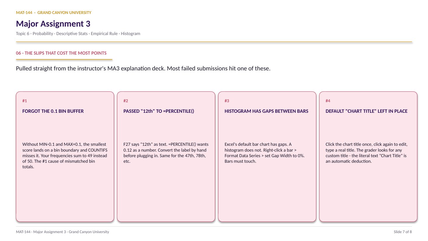
Common slips
Four mistakes that cost the most points.
The percentile-text trap and the typed-stats trap are the two biggest point-killers on this tab. Read your formula bar before you submit.
01
Typed “12th” as text into PERCENTILE.
The label in F27 reads “12th” but the function needs the decimal: =PERCENTILE(D14:D63, 0.12). If you typed the text string, the cell shows #VALUE! or #NUM!. Convert each label by hand before typing the formula.
02
Confused Empirical Rule with Chebyshev.
Cell 5b wants the 68% interval - one SD on each side of the mean. Not 75%, not 95%, not 99.7%. Chebyshev is the conservative bound for any distribution; Empirical assumes near-normal. Use Empirical here. G36 = H18 - H20 and G37 = H18 + H20.
03
Typed the statistics by hand instead of using functions.
Every cell in the G18:I21 grid must read =AVERAGE(...), =MEDIAN(...), =STDEV(...), or =MAX(...) - MIN(...) in the formula bar - not a typed-in number. Self-check needs both: right answer AND a real function.
04
Generic written answer in F43 with no specific bounds.
“Tutoring helped students do better” loses points. The grader wants your actual G36 and G37 values quoted, the “about 34 of 50” Empirical Rule framing, and an explicit yes / no on whether tutoring helped. Cite the numbers; don’t paraphrase the concept.
Application & connection
This is Topic 5 descriptive stats + Topic 6 empirical rule in one tab.
If the stats feel distant, the Topic 6 cheat sheet lists every formula you need in one place. If the empirical rule feels distant, Topic 6 Review Question 4 walks through a similar bell-curve interval calculation.
The output of this tab - the 50 numbers in D14:D63 - is the input Component 2 (Visualization) uses to build the frequency distribution and histogram. Get this tab right and the histogram side gets easier.