TOPIC 6 · DQ 1 / Probability / discussion question

01Simulate. Count. Compare. Converge.

An n-sided die in your spreadsheet, rolled 1,000 times in one column and 4,000 times in another. The empirical probabilities jitter around the theoretical 1/n — tighter on the bigger sample. The Law of Large Numbers, drawn in your own data.

Discussion · 5 pts Initial post Wed · replies Sun =RANDBETWEEN Law of Large Numbers

▸ The why · 7-slide reference

1 / 7

↓ Download .pptx

Step 1 · materials

Download the worksheet

Topic_6_DQ_1.xlsx

XLSX 5 pts v · spring 26

Step 2 · walkthrough

Watch the click-by-click

Every keystroke for both tables. The Scribe walkthrough lands here once recorded; for now, the Excel template above is your working surface.

SCRIBE.HOW · YOUTUBE

Step-by-step walkthrough

Coming soon. Check back after the Scribe is recorded.

Same walkthrough, two modes. Use whichever helps you today.

Open the Probs tab. Type your name in cell C1 — the formula in A4 uses your name's length to pick a number of sides n in the range 10 to 15. Now autofill the rolls: select C4 and drag down to C1003 (1,000 rolls for Table 1); select D4 and drag down to D4003 (4,000 rolls for Table 2). Then fill in the empirical probability column H with =G4/$A$7 for Table 1 (and the corresponding formula using $A$10 for Table 2), and the theoretical probability column I with =1/$A$4. Average the absolute deviations in J19 (Table 1) and I38 (Table 2). Finally, type any character in the Response cell K30 and hit Enter five times — each press re-rolls the whole sheet. Record the five pairs of average deviations and write a short response in K30 comparing the two table sizes. New to the cell color codes? See the legend.

§1 · Type your name

Pick the die.

Cell A4 computes the number of sides from your name's length. Two students with the same name length get the same die; different names produce different dies.

§2 · Autofill rolls

1,000 + 4,000.

Fill C4:C1003 for Table 1 and D4:D4003 for Table 2. The $ in $A$4 keeps the formula pointing at the right cell as it copies down.

§3 · Empirical + theoretical

Frequency / rolls, and 1 / sides.

Column H: empirical (=G4/$A$7). Column I: theoretical (=1/$A$4). Both denominators absolute-referenced so the copy-down works.

§4 · Average deviation

One number per table.

Compute =AVERAGE(J4:J18) in J19 for Table 1 and the corresponding average in I38 for Table 2. These two numbers tell the story.

§5 · Rerun + response

Type, Enter. Five times.

Each press of Enter in the Response cell K30 re-rolls everything. Record the five pairs of averages, then write the response: Table 2's average is consistently smaller.

The die

Name-keyed, 10 to 15 sides.

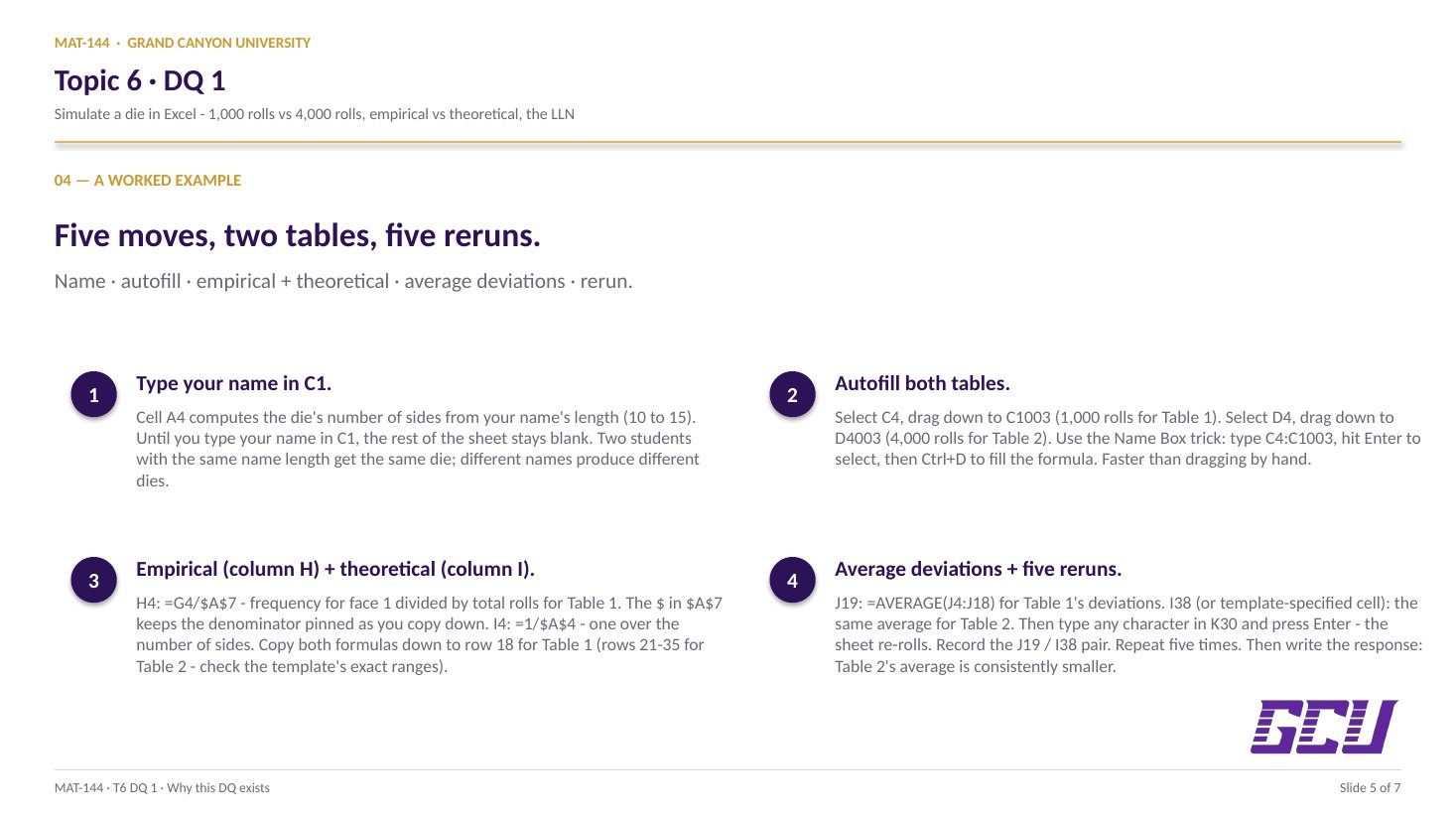
The die has between 10 and 15 sides, and the exact number is set by a formula in cell A4 that depends on your name: =MOD(LEN(C1)*5857,6)+10. Two students with the same name length get the same die; a different name produces a different die. Until you type your name in C1, the rest of the sheet sits blank.

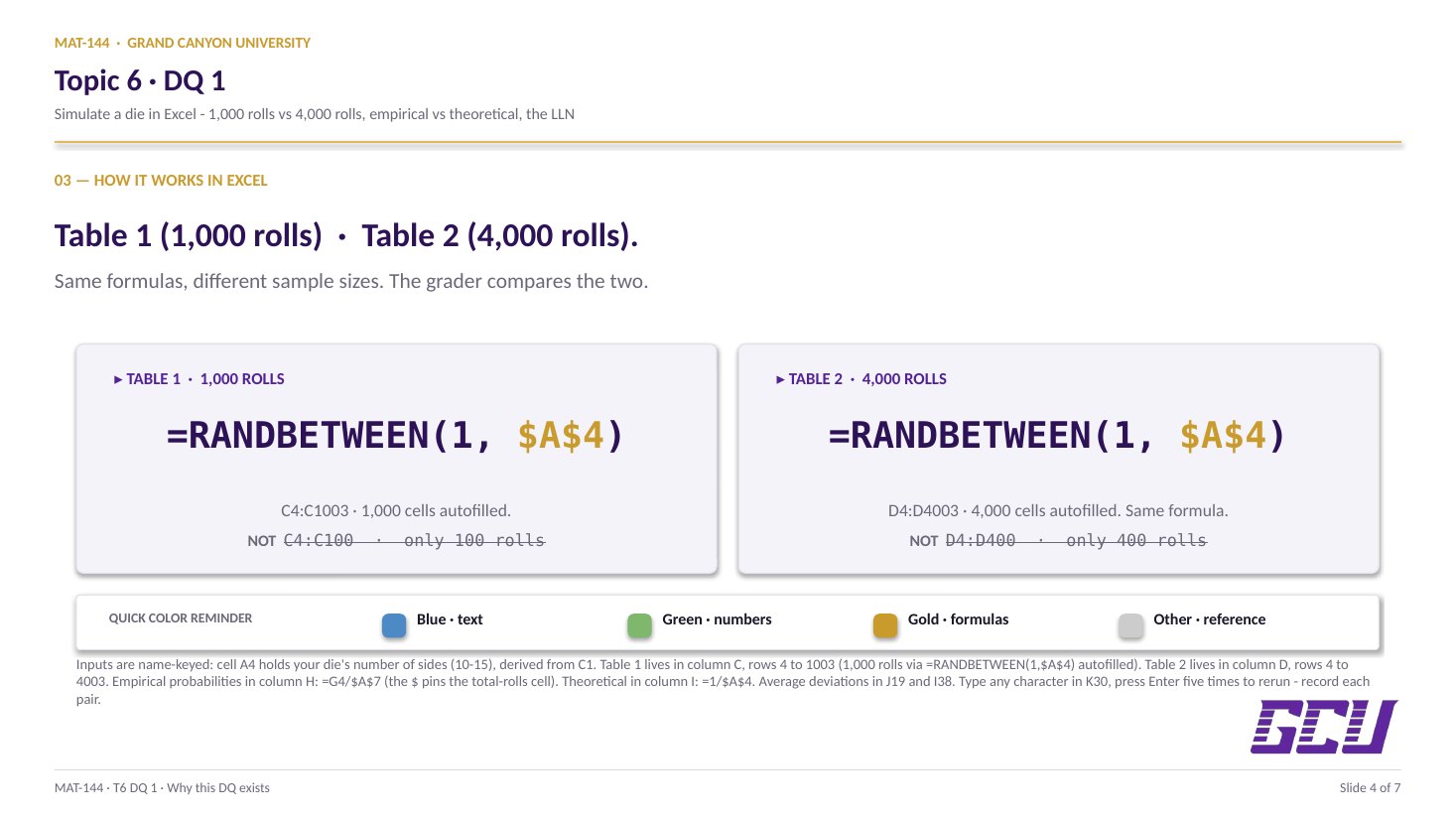
The roll itself is generated by Excel's =RANDBETWEEN(1, $A$4) in cells C4 and D4. Each time you trigger a recalculation (the easiest way: type any character in the "Response" cell K30 and press Enter), every RANDBETWEEN in the sheet re-rolls. Think of it as rolling the die fresh every time the sheet recalculates.

Autofill

1,000 in column C, 4,000 in column D.

The simulation needs two large columns of rolls: 1,000 rolls in column C (rows 4 through 1003) for Table 1, and 4,000 rolls in column D (rows 4 through 4003) for Table 2. The formula =RANDBETWEEN(1, $A$4) already lives in C4 and D4; your job is to autofill it all the way down.

Two efficient ways. (i) Double-click the fill handle — select the cell, hover over the bottom-right corner until the cursor turns into a black plus, double-click; the formula fills down to the bottom of the adjacent data automatically. (ii) Type a range into the Name Box (top-left of the workbook): C4:C1003, hit Enter, then Ctrl+D to fill the formula. Repeat for column D with the range D4:D4003.

The $ in $A$4 matters here. As the formula copies down, the absolute reference keeps pointing to A4 (the "number of sides" cell) instead of drifting to A5, A6, A7… which would all be blank.

C4: =RANDBETWEEN(1, $A$4)
autofill C4:C1003 · 1,000 rolls for Table 1

D4: =RANDBETWEEN(1, $A$4)
autofill D4:D4003 · 4,000 rolls for Table 2

Two columns, two table sizes. The same formula in both, copied to different depths.

Empirical probability

=G4/$A$7, denominator locked.

The empirical probability of a face is the share of rolls that came up that face. The =COUNTIF formula in column G already tallies each face's frequency for Table 1; your job is to convert that frequency into a probability by dividing by the total number of rolls.

The total lives in cell A7 (Table 1) and A10 (Table 2). Your formula for the first row of Table 1 in H4:

=G4/$A$7

Lock the denominator with $A$7 so that when you copy the formula down to H5, H6, … the frequency in column G drifts forward but the total stays anchored on the same denominator. Copy down through H18 for the 15 possible faces (Excel just fills blank rows below if your particular n is smaller than 15). Repeat for Table 2 in column H rows 23 onward, using $A$10 as the denominator.

H4 = G4 / $A$7 empirical, Table 1
I4 = 1 / $A$4 theoretical, both tables
J19 = AVERAGE(J4:J18) avg deviation, Table 1

Three formulas, two locked denominators, one summary number per table.

Theoretical probability

=1/$A$4, one over n.

The theoretical probability of each face on a fair n-sided die is, by definition, 1/n — the favorable-over-total ratio from Lesson 1, with one favorable outcome out of n equally-likely total outcomes. The formula in cell I4:

=1/$A$4

Again, lock the denominator with $A$4 so copying down keeps the same number of sides in every row. The theoretical probability is the same for every face (that is what "fair die" means), so the column shows the same value repeated, and the empirical column to its left will jitter around it.

Column J already computes the absolute deviation |empirical − theoretical| for each face. Your last calculation is to average those deviations in cell J19 for Table 1 (formula =AVERAGE(J4:J18)) and in cell I38 for Table 2. The average deviation is the single number that summarizes how close the simulation got to the math.

Convergence

4,000 rolls beats 1,000.

One run is not enough. Type any character in the Response cell K30 and press Enter five times. Each press re-rolls every die in the sheet, recomputes the frequencies, and updates the average deviations. Record the five Table 1 and Table 2 averages on paper or in a scratch corner of the sheet.

The pattern you should see: Table 2's average deviation is consistently smaller than Table 1's. 4,000 rolls produce a simulation that agrees more closely with the theoretical 1/n than 1,000 rolls do, and the pattern is reliable across the five reruns (not just a coincidence of one trial). Bigger samples shrink the gap.

That is the Law of Large Numbers at work in your spreadsheet. The same principle predicts that 40,000 rolls would shrink the gap further still, 400,000 further still, and so on without bound — the empirical probability converges (in the limit) to the theoretical one. This is the same effect that lets a casino price its games on the long-run expected value despite any individual gambler winning big now and then.

Common slips

Five mistakes this DQ punishes.

The locked-denominator slip and partial-autofill slip are the most common. Read these before you submit.

01

Forgot the $ in $A$7 (or $A$4).

When you copy the empirical formula down to H5, H6, …, you want the frequency in column G to drift forward but the denominator to stay anchored on the same total. Without the absolute reference, Excel uses A8, A9, A10 (all blank) as the denominator and you get #DIV/0! errors or wildly wrong probabilities.
02

Autofilled only part of the column.

Table 1 needs 1,000 rolls in C4:C1003; Table 2 needs 4,000 rolls in D4:D4003. If you stop at row 100 or 500, the COUNTIF tallies are smaller than intended and the empirical probabilities drift further from the theoretical. Use the Name Box trick: type C4:C1003, hit Enter to select the range, then Ctrl+D to fill the formula down.
03

Typed the theoretical probability as a decimal instead of a formula.

For a 12-sided die, 1/12 ≈ 0.0833, but the grader expects a formula referencing $A$4, not a hardcoded decimal. Use =1/$A$4. The advantage: if you somehow change the die (e.g., trying a different name), the theoretical column updates automatically.
04

Recorded only one run of the average deviations.

Task 5 explicitly asks you to rerun the sheet five times and record the averages each time. A single run could be a lucky or unlucky roll; five runs show the pattern is reliable. Type any character in K30 and hit Enter to trigger a recalculation.
05

Wrote the response saying Table 1 (1,000) is more accurate than Table 2 (4,000).

It is the other way around. Larger samples produce smaller average deviations from the theoretical 1/n. The Law of Large Numbers predicts that more rolls = tighter agreement. Your five reruns should confirm Table 2's average is consistently smaller than Table 1's.

Application & connection

From this DQ into DQ 2 and the topic finale.

This DQ is the empirical half of Topic 6. Lessons 1 through 5 built the theoretical machinery — counts, addition rule, permutations and combinations, expected value — each computed from the structure of the experiment. Lesson 6 and this DQ swing the other way: take the same experiment, run it many times, and compare the data with the math.

The bridge to DQ 2 is the question of scale. DQ 1 stays inside a single experiment and asks how its empirical probability converges as the sample grows. DQ 2 broadens that to compound events and to the long-run interpretation of expected value — the topic-finale move that ties counting, probability, and decision-making into one number.

In practice, every experimental science runs on the same loop: write down what the math predicts, run the trial many times, compare. The closer your data agrees with the math, the more confidence you have in both. The Law of Large Numbers is the guarantee that, given enough trials, the agreement must arrive.