TOPIC 4 · MAJOR ASSIGNMENT 2 · COMPONENT 03/ Financial Literacy / major assignment / credit cards
03Pay the minimum, watch the years pile up.
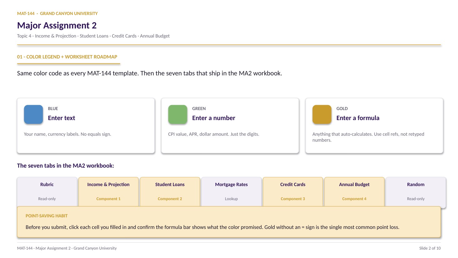
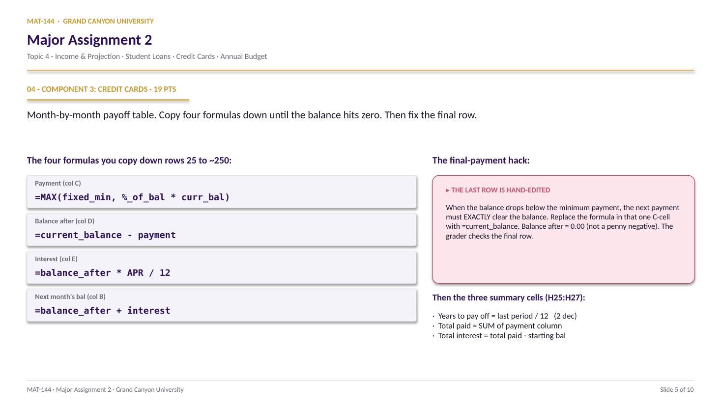
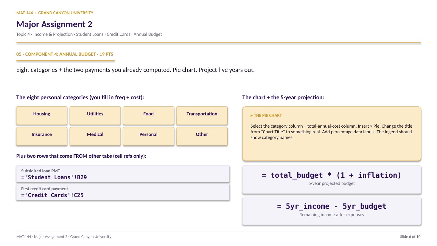
Build a month-by-month payoff table from a personalized balance and APR. The payment is MAX(fixed-min, percent-of-balance). Hand-edit the final payment to exactly clear the balance. Summarize the time, total paid, and total interest.
Major Assignment · 19% of Excel
524 rows reserved
=MAX(C13, C17*B_row)
A 7-page MA2 Walkthrough PDF covers all four components in the same hint depth as this page. Useful if you'd rather print, annotate on paper, or keep it open on a second screen while working in Excel.
Walkthrough video coming in a future recording. Until then, work from the slideshow above and the printable PDF.
SCRIBE.HOW · YOUTUBE
≡
Step-by-step walkthrough
Coming soon. Check back after the Scribe is recorded.
▸
Video walkthrough
Coming soon. Work from the slideshow and printable PDF until then.
The Topic 4 Review Q2 video walks the same monthly-statement bookkeeping MA2 C3 asks you to run on your credit-card tab. Two moves in order: interest = prior balance × (r/12), then new balance = beginning − payments + purchases + interest. Interest is charged only on the prior balance; new purchases don’t accrue yet. Same math, worked on video — swap in your own APR and transactions as you go.
Same walkthrough, three modes.Pick the one that lands for you today.
ORIENT
· the tab
Six inputs, one long table, three summaries.
The six green parameter cells drive everything. The payoff table is one formula per column, copied down. The three summary cells live up top in column H.
Cell A3 spawns a personalized problem statement (with your name). Green cells C13:C18 hold the six input parameters: APR, starting balance, payments per year, fixed minimum, percent-of-balance, and the larger fixed min. Most are pre-filled; you confirm them. Then the real work is the payoff table starting at row 25.
§1 · Inputs
C13:C18 - the six green parameters.
APR (C13), starting balance (C14), payments per year (C15), min payment $ (C16), % of balance (C17), fixed min $ (C18). Confirm each one matches the prompt in A3.
§2 · Payoff table
B25:E? - one row per month.
Five columns: month, current balance, payment (MAX rule), balance after, interest. Each row references the previous. Copy down until the balance hits zero.
§3 · Final row
Hand-edit so the last balance is $0.00.
Copy-down will leave a small negative or positive balance. Hand-edit the final payment to exactly zero the balance. This is the most common point-loss on the whole tab.
§4 · Summaries
H25 years · H26 total · H27 interest.
Years = last month / 12. Total = SUM of the payment column. Interest = total - starting balance. Format years as Number with 2 decimals, dollars as Currency.
CONCEPTS · six things to know
The four moves that drive every row.
MAX rule on the payment. Subtract for balance-after. Multiply by APR/12 for interest. Carry the new total into the next row.
01
MAX
Every payment is MAX(fixed, percent × balance).
The credit-card minimum payment is the larger of two values: a fixed dollar floor (like $25) and a percent-of-balance amount (like 2% of the current balance). Excel: =MAX(C13, C17 * B25) for row 25, then the relative reference walks the table down.
Without MAX(), the percent-of-balance payment shrinks to nothing and the loan never pays off. With MAX(), the fixed minimum eventually kicks in once the balance is low enough - that’s the lever that finishes the payoff.
=MAX($C$13, $C$17 * B25)
Fixed min OR percent-of-balance - larger wins.
Anchor C13/C17 with $ signs; B25 walks down.
02
Balance after
Current balance minus payment.
Cell D25: =B25 - C25. The “balance after” column shows what’s left of the loan after this month’s payment. The math is intuitive - you pay C25, so the balance drops by exactly that much.
Format as Currency. The interest hasn’t been added yet (that’s the next column), so this is the lowest the balance gets all month - the moment right after you paid the bill, before next month’s interest hits.
=SUM(E21:E28)
=Switch on
SUMFunction name
( )Argument hold
E21:E28Range arg
03
Interest
Monthly interest = balance-after × APR / 12.
Cell E25: =D25 * $C$13 / 12. APR is annual; the monthly rate is APR / 12 (or APR / payments_per_year if it isn’t 12). Multiply the balance-after by that rate to get the interest that’s charged before next month’s payment.
Format as Currency. The interest is added back into next month’s current balance - that’s how the credit card “earns” money even when you’re paying every month. The slower you pay, the more interest rolls forward.
Cell by cell
=(E21+E22+E23+…+E28)/8
⟶
Range, scales freely
=AVERAGE(E21:E28)
04
Carry
Next row’s current balance = D + E from the previous row.
Cell B26: =D25 + E25. The balance after the payment, plus the interest charged on that balance, is what carries into month 2. That sum is more than the balance-after, because interest just got added. The loop continues.
Now copy row 25 (B25:E25) down. Excel’s relative references should walk B → C → D → E forward for every month. Watch the balance column. When it hits zero, stop.
a + b
↓
a+b
Plus
a − b
↓
a-b
Minus
a × b
↓
a*b
Asterisk
a ÷ b
↓
a/b
Slash
ab
↓
a^b
Caret
05
Final
Hand-edit the last payment to exactly clear the balance.
Copy-down will leave the last row imperfect - the MAX() rule keeps charging the fixed minimum even when only a few cents are owed. Find the last row where the balance before payment is positive. Replace its payment formula with the current balance value, so the balance after lands at exactly $0.00.
Self-check: does the last “balance after” cell read $0.00 with no minus sign and no leftover cents? If yes, you’re done. If not, edit again. The grader checks this cell specifically.
Stored in cell
1.1428571428571428
Displayed (2 dec.)
1.14
06
·
B8+C8TEXT · LABEL
— PRESS = —
=
=B8+C815
Summary
Years, total paid, total interest - three cells.
H25 (years to pay off):=last_month_number / 12. Two decimals. H26 (total paid):=SUM(C25:Clast). Currency. H27 (total interest):=H26 - C14 - total paid minus the starting balance. Currency.
If your total interest is bigger than your starting balance, you’re reading the result right - that’s the headline of the whole credit-card story.
Common slips
Five mistakes that cost the most points.
The instructor explicitly flagged the final-payment hand-edit as the most common point-loss on the whole assignment. Two minutes of cleanup at the end matters.
01
Final balance isn’t exactly $0.00.
The instructor’s #1 flag. Copy-down will leave a few cents negative or positive. Hand-edit the last payment cell: replace the MAX() formula with the exact value needed to land at $0.00 balance after. The grader checks this specific cell.
02
Forgot the MAX() rule on payment.
If your payment column just uses =$C$17*B_row, the percent-of-balance payment approaches zero and the payoff never finishes. Wrap it: =MAX($C$13, $C$17*B_row).
03
Wrong divisor on interest.
APR is annual; the monthly rate is APR / 12. If your total interest is roughly 12x what it should be, you forgot the /12 in the interest column.
04
Total interest subtracted the wrong cell.
Total interest is =H26 - C14 (total paid minus starting balance in C14, not the last current balance, not the new principal). If you got a tiny number near zero, you subtracted the wrong cell.
05
Years formatted as Currency or %.
Cell H25 (years to pay off) is a Number with 2 decimals. Not Currency, not Percentage. If it reads $8.42 or 842%, fix the format on that one cell.
Application & connection
This is amortization with a moving payment.
This component is loan amortization with a twist: the payment isn’t fixed, it shrinks as the balance shrinks. That’s why credit cards on minimum payments take years - the MAX() rule keeps the payment small while the interest keeps compounding on whatever’s left.
The Component 2 PMT formula assumes a constant payment over a fixed term; this tab gives up the constant payment to model how credit-card statements actually work. The same APR-divided-by-n logic appears in both tabs - that’s the rate-per-period pattern from Topic 3 Lesson 4 (Compound Interest) and Topic 4 Lesson 3 (Loans).
The first month’s payment (cell C25) feeds the budget tab (Component 4) by cell reference. Get the MAX() rule right and the Annual Budget reads the correct row automatically.