TOPIC 4 · DQ 2 / Loans / discussion question

02The loan calculator. Built by hand.

One Loans tab, one financial calculator row. Plug L2's amortization formula into Excel by hand — randomized inputs, your formula, three answer cells. The same finger memory that powers MA2.

Discussion · 5 pts Initial post Fri · replies Sun PMT formula No =PMT()

▸ The why · 7-slide reference

1 / 7

↓ Download .pptx

Step 1 · materials

Download the worksheet

Topic_4_DQ_2.xlsx

XLSX 5 pts v · spring 26

Step 2 · walkthrough

Watch the click-by-click

The instructor's note on the sheet: “There is no video for this one, it is just like Topic 3 DQ 1.” Same formula shape, opposite direction — lean on T3 DQ1's Scribe if you need one. The Excel template above is your working surface.

SCRIBE.HOW · YOUTUBE

Step-by-step walkthrough

Coming soon. Check back after the Scribe is recorded.

Same walkthrough, two modes. Use whichever helps you today.

Open the Loans tab. Type your name in the blue cell at the top — the inputs (P, r, n, t) for the calculator row are generated from your name, so your version is unique. The instructions in cell B18 will rewrite themselves with your specific numbers (e.g. "Compute the monthly payments to pay back a loan of $X over Y years at Z% APR"). Type the amortization formula into H17, then the two arithmetic cells (I17, J17) for Total Paid and Interest. New to the cell color codes? See the legend.

§1 · Loans tab

Single calculator row.

P, r, n, t in B17:E17 (auto-randomized). Three formula cells you fill: H17 (PMT), I17 (Total), J17 (Interest).

§2 · The formula

PMT = P·(r/n)/(1−(1+r/n)^(−n·t)).

L2's amortization formula, verbatim. Excel: =B17*(C17/D17)/(1-(1+C17/D17)^(-D17*E17)).

§3 · Two more cells

Total + Interest.

Total = PMT × n × t. Interest = Total − P. Both arithmetic, both fall out of H17.

§4 · No =PMT()

Built-in is off-limits.

Same rule as T3 DQ1. Type the formula manually with cell references. The self-check distinguishes "right answer typed" from "right answer computed."

Loans tab

Single row, four randomized inputs.

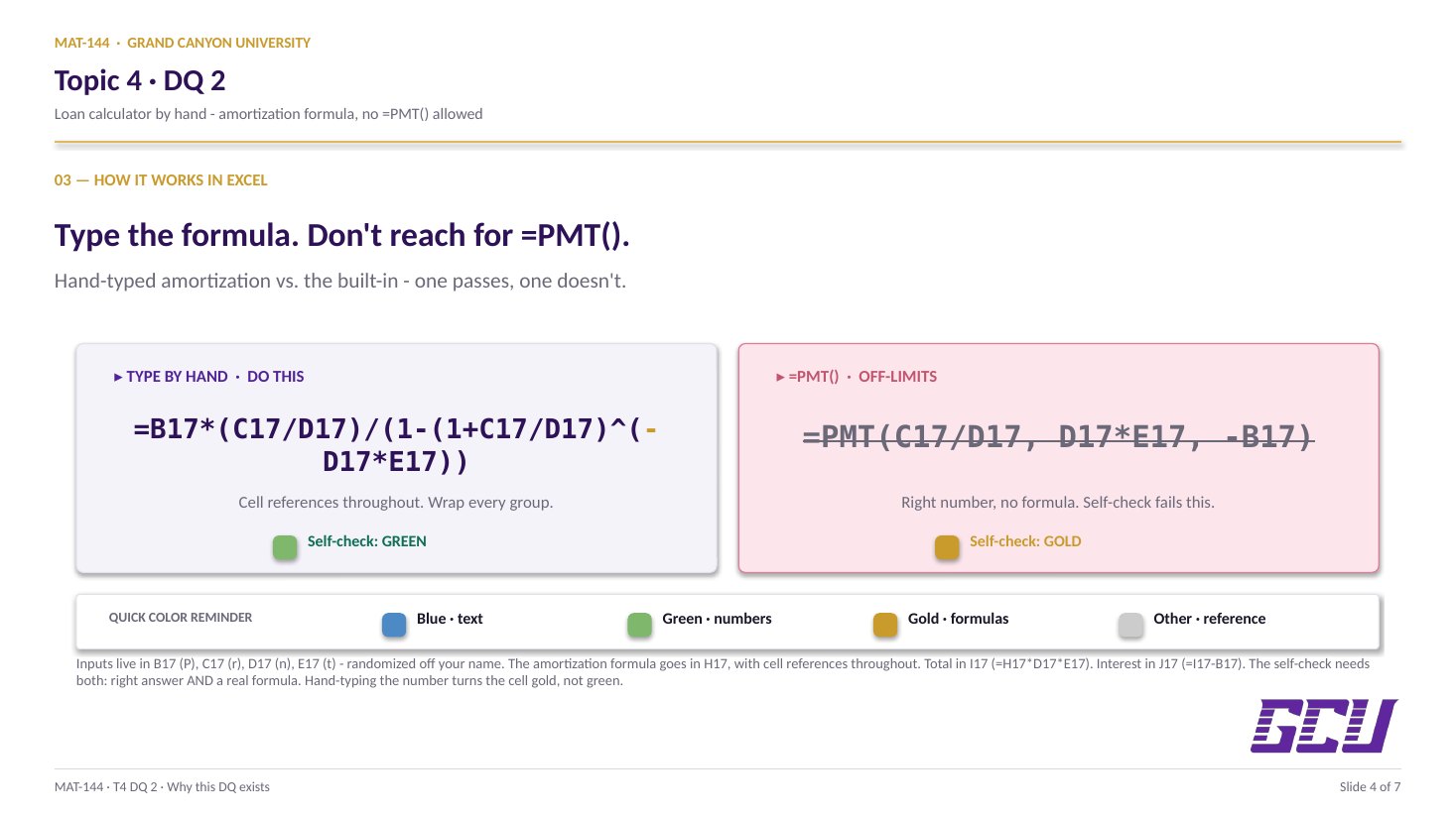
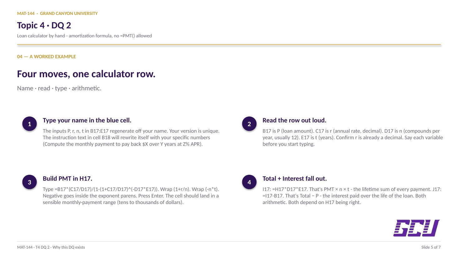
One row, four randomized inputs. The Loans tab's calculator lives at row 17. Four input cells get filled automatically based on your name (cells B17 through E17): P (loan amount), r (APR as a decimal), n (compounding periods per year), and t (term in years).

The instructions in cell B18 are a self-rendering string: once you type your name in cell C2, the prompt rewrites itself with your specific numbers, e.g. "Compute the monthly payments to pay back a loan of $X in Y years at an APR of Z." That's the problem you're solving. Three computation cells (H17, I17, J17) wait for your formulas.

Like T3 DQ1: every student's randomized values are different, so you can't copy from a friend's sheet. The math is identical; the numbers are yours.

The formula

Amortization, typed by hand.

The amortization formula in Excel syntax. The legend printed on the sheet shows: PMT = P×(r/n) / (1 − (1 + r/n)^−n·t). In Excel with cell references, that becomes:

=B17*(C17/D17)/(1-(1+C17/D17)^(-D17*E17))

Watch every parenthesis. The exponent (-D17*E17) is in its own parens because Excel evaluates ^ right-to-left and treats ^-D17*E17 very differently from ^(-D17*E17). Same rule that bit students on T3 DQ1's Problem 2.

The denominator is (1 - (1+r/n)^(-n*t)); the numerator is P*(r/n). They divide. The result is your monthly payment. Format the cell as currency with two decimals and the value will read $X.XX.

Total + Interest

Two arithmetic cells fall out from PMT.

Two arithmetic cells fall out from PMT. Once your monthly payment is computed in cell H17, the next two columns are simple:

Total Paid (cell I17): =H17*D17*E17 — that's PMT × n × t, the sum of every payment over the full term. Same shape as T3 DQ1's annuity formula's "total invested" cell.

Interest Paid (cell J17): =I17-B17 — the total paid minus the original loan amount. That subtraction isolates the cost of borrowing — everything you handed back to the bank beyond the principal you originally received.

Both should format as currency automatically if you formatted PMT correctly. Sanity check: interest paid is always less than total paid, and always less than P times the rate times t (which would be simple-interest-only).

PMT × n × t

↓

=H17*D17*E17

Total Paid
(every payment, summed)

Total − P

↓

=I17-B17

Interest Paid
(cost of borrowing)

=PMT(...)

built-in

rejected by this DQ
different param order
different sign convention

=B17*(C17/D17)/(1-(1+C17/D17)^(-D17*E17))

manual formula

required by this DQ
matches L2's textbook formula
same shape used in MA2

Rule

Why =PMT() is off-limits.

The DQ instructions on cell F21 are explicit: do not use the built-in =PMT() or =FV() functions. You have to type the amortization formula manually with cell references and arithmetic operators.

Three reasons (same as T3 DQ1). First: writing the formula yourself is the actual skill the DQ is testing. Second: Excel's =PMT() uses a different parameter order than the textbook formula and returns negative numbers under some sign conventions — using it without understanding the convention is a recipe for sign errors. Third: Major Assignment 2 reuses the same formula by hand for four different loan types. Manual fluency here = MA2 in half the time.

The self-check on the Loans tab catches this: a typed number that happens to be right gets flagged separately from a correct formula result. Both have to be green for credit.

Connection

Same formula. Four loans in MA2.

Where this formula goes next: Major Assignment 2. MA2 has four loan analyses — an auto loan, a credit card balance, a student loan, and a mortgage. Each one asks for the monthly payment, total paid, and total interest, plus a brief written analysis of whether the loan is affordable given a budget.

That budget? It came from T4 DQ1. So the two DQs in Topic 4 are MA2's two halves: DQ1 builds the budget, DQ2 builds the loan calculator that has to fit inside it. The written analysis in MA2 is the comparison between them.

If you've completed DQ1 and DQ2 cleanly, MA2 is mostly the same formulas applied to four different scenarios + a few paragraphs of analysis. The hard part is the spreadsheet work — which you just did.

Common slips

Five mistakes this DQ punishes.

Read these before you submit. The exponent-parens slip and the missing negative sign are by far the most common.

01

Used =PMT().

Explicitly off-limits for this DQ. The instructor catches it via the self-check; the cell turns gold (right number, no formula) instead of green. Type the formula manually with cell references and arithmetic operators.
02

Wrong parentheses on the exponent.

(1+r/n)^-n*t means (1+r/n)^-n × t — totally different from (1+r/n)^-n×t. Wrap the exponent: (1+r/n)^(-n*t). Always.
03

Missed the negative sign in the exponent.

The amortization formula uses (1+r/n)^(-n*t), NOT (1+r/n)^(n*t). The negative makes the denominator 1 minus a small number instead of 1 minus a huge number. Drop the negative and your monthly payment comes out negative or wildly wrong.
04

Used the rate as a percent instead of a decimal.

The randomized r in the green cells is already in decimal form (e.g. 0.06 for 6%). Don't type =B17*(6/12)/... with the integer 6 — use the cell reference C17 directly. If your monthly is $1.4 million, this is why.
05

Multiplied wrong order in Total Paid.

Total Paid = =H17*D17*E17 (PMT × n × t). Don't swap n and t with year inputs from somewhere else. PMT is your computed monthly value, n is compounds per year (12 here), t is years. The product is the lifetime sum of every payment.

Application & connection

From this DQ into MA2.

This DQ is the loan-side mirror of T3 DQ1's Problem 4. There you solved the annuity formula for the monthly deposit needed to reach a savings goal; here you solve the amortization formula for the monthly payment needed to pay back a loan. Same algebraic shape, opposite direction. If T3 DQ1 felt clean, this should too.

The formula you typed today — =B17*(C17/D17)/(1-(1+C17/D17)^(-D17*E17)) — is exactly the Excel call you'll need in Major Assignment 2 for each of the four loan types (auto, credit card, student, mortgage). Different P, r, t per scenario; identical formula. Get fluent here, save time there.

The instructor's note: "There is no video for this one, it is just like Topic 3 DQ 1." If you want a walkthrough, the Scribe on T3 DQ1 covers the same formula shape — just substitute "monthly payment" for "monthly deposit" in your head.