TOPIC 4 · DQ 1 / Loans / discussion question

01Build a budget. Then put loans against it.

Six categories, twelve rows each, two tabs that talk to each other. The prerequisite check before you decide what an auto loan, credit card, student loan, or mortgage costs you can actually carry.

Discussion · 5 pts Initial post Wed · replies Sun =SUM =Budget!C23

▸ The why · 7-slide reference

1 / 7

↓ Download .pptx

Step 1 · materials

Download the worksheet

Topic_4_DQ_1.xlsx

XLSX 5 pts v · spring 26

Step 2 · walkthrough

Watch the click-by-click

Every keystroke for both tabs. The Scribe walkthrough lands here once recorded; for now, the Excel template above is your working surface.

SCRIBE.HOW · YOUTUBE

Step-by-step walkthrough

Coming soon. Check back after the Scribe is recorded.

Same walkthrough, two modes. Use whichever helps you today.

Open the Budget tab. Type your name in the blue cell at the top, then enter your monthly expenses across the six category columns. Subtotal each column with =SUM(...), then compute the percent of total in the next column with =part / C$23. Insert a pie chart and a bar chart. Then jump to the Percentage Change tab and let the live-linked budget total drive the "income = 150% of budget" calculations. New to the cell color codes? See the legend.

§1 · Budget tab

Six categories, =SUM, percentages.

Enter dollar amounts in F16:K27. Subtotal each column with =SUM. Compute percent of total with part/total — pin the denominator with $.

§2 · Charts

Pie + bar.

Two charts on the Budget tab. Pie shows the percentage breakdown; bar shows the dollar amounts. Add titles + axis labels.

§3 · Cross-tab link

=Budget!C23.

On the Percentage Change tab, pull the monthly total forward via =Budget!C23. Live-linked — change Budget, this follows.

§4 · Percent math

150% of budget · +10% bump.

Income = 1.5 × budget. Budget % of income = budget/income. Bump income by 10%; the new budget grows by exactly 10% too (linearity).

Budget tab

Six categories, twelve rows each.

Budget tab data entry. The grid lives in columns F–K, rows 16–27. Six categories across the top — Housing, Food, Utilities, Auto, Recreation, Other — with up to twelve line-item rows under each. You enter the dollar amount for each individual expense in the appropriate cell.

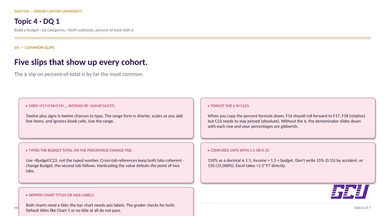
Format as currency with two decimals ($12.34, not 12.34 or $12). Use Format Cells → Currency, or just type the dollar sign as you go. The instructor's sheet will check formatting, not just values.

You don't need to fill every row. If you only have three items in Recreation, leave the other nine rows blank — the SUM formula in the next concept card handles blank cells gracefully. The reason the table goes to row 27 instead of, say, row 22 is to give you room to add line items later without breaking the formulas.

Subtotals

=SUM over a range, six times.

The =SUM formula does the heavy lifting. For the Housing subtotal in cell C17, you write =SUM(F16:F27). That's "sum every value in column F from row 16 to row 27." Repeat the pattern for Food (column G), Utilities (column H), Auto (column I), Recreation (column J), and Other (column K) — six SUMs, one per category subtotal.

Then the Monthly Total in C23 sums the six subtotals: =SUM(C17:C22). (Or equivalently =SUM(F16:K27) over the entire grid — either gives the same number.)

Why a range, not cell-by-cell. You could write =F16+F17+F18+...+F27 for each subtotal, but that's twelve plus signs you'd have to type six times. The range form F16:F27 handles blank cells, scales if you add a row, and is a single keystroke shorter than the addition. This is exactly L2's distinction in T3's lesson — scale freely, the formula doesn't care how many cells are populated.

Percent of total

Part / whole, with the $ trick.

Percent of total = part / whole. For the Housing percentage in D17, you write =C17/C$23 — that's the housing subtotal divided by the monthly total.

The dollar sign matters. The $ in C$23 is an Excel absolute reference: when you copy the formula down to D18, D19, D20, D21, D22, the C17 part rolls forward to C18, C19, etc. (relative reference, no dollar sign), but the C$23 stays anchored to row 23 (absolute reference, dollar sign). Without the $, copying the formula would shift the denominator down with each row and your percentages would be gibberish.

Sanity check: D24 should equal 100%. The sheet's check cell adds your six percentages and confirms they total to 1.00 (or 100%). If they don't, either a percentage formula is missing or you forgot the $ in the denominator. Format the percentage column with the % button (or Format Cells → Percentage) with two decimals.

Cross-tab

Pull Budget!C23 into the next tab.

Pulling Budget!C23 into the next tab. The Percentage Change tab opens with one question: "What's your monthly budget?" You don't re-type the number from the Budget tab. You write a cross-tab reference: =Budget!C23.

That syntax (SheetName!CellAddress) makes the cell live-linked. Change anything on the Budget tab — add a Recreation expense, raise your rent — and the Monthly Budget cell on the Percentage Change tab updates automatically. Same goes downstream: your "income = 150% of budget" calculation, your "new income at +10%" projection, your "percent increase in budget" — they all follow.

Why this matters beyond the DQ: in any real budget tracker (yours, your accountant's, a startup's P&L), data lives on one sheet and analyses live on another. Cross-tab references are how spreadsheets stay coherent as they grow.

Percent change

Income +10% → budget +10%.

The Percentage Change tab is T2 percent math applied to your own budget. Five quick calculations, all driven by the live link to the Budget tab.

1. Income at 150%. If your monthly income is 150% of your budget, then income = 1.5 × budget. Excel: =1.5*F7 where F7 holds the live-linked budget total.

2. Budget as % of income. Reverse direction: =F7/F9. With the 1.5× relationship that's exactly 0.6667, or 66.67%.

3. Income +10%. New income = old income × 1.10: =F9*(1+10%). Excel accepts the 10% notation directly — it converts to 0.10 under the hood.

4. New budget at the new income. If the "budget is 60-some-percent of income" ratio holds, new budget = ratio × new income, i.e. =F12*F15. (Equivalently, new budget = new income / 1.5.)

5. Percent increase in budget. The classic percent-change formula: =F18/F7-1 — new over old, minus 1. Format as percentage with two decimals; because the budget grew exactly proportionally to income, this should land at 10.00%.

Common slips

Five mistakes this DQ punishes.

Read these before you submit. The absolute-reference slip on the percent column and the cross-tab shortcut on the second tab are by far the most common.

01

Used =F17+F18+F19+... instead of =SUM(F16:F27).

Twelve plus signs is twelve chances to typo. Range form is shorter, scales as you add line items, and ignores blank cells. Use the range.
02

Forgot the $ in C$23.

When you copy the percent formula down to D18, D19, D20…, you want C17 to roll forward to C18 (relative) but C23 to stay anchored (absolute). Without the $, the denominator shifts down with each row and your percentages are gibberish.
03

Typed the budget total on the Percentage Change tab.

Use =Budget!C23, not the typed number. Cross-tab references are how spreadsheets stay coherent — change Budget, the second tab follows. Hardcoding the value defeats the whole point.
04

Confused 150% with 1.5 (or wrote it as 0.15).

150% as a decimal is 1.5. So income = 1.5 × budget. Don't write 15% (=0.15) by accident, or 150 (=15,000%). Excel accepts =1.5*F7 directly.
05

Skipped chart titles or axis labels.

Both charts need a title (Insert → Chart Title) and the bar chart needs axis labels (Insert → Axis Title). The instructor will check for these. Default titles like "Chart 1" or no title at all are not acceptable.

Application & connection

From this DQ into the loans you just learned.

This DQ is the input to every loan you'll ever consider. The four lesson types you just learned — auto loans (L3), credit cards (L4), student loans (L5), mortgages (L6) — all output a fixed monthly payment M. The decision "can I afford this loan?" is one comparison: does M fit inside my budget for that category?

The financial-planning rules of thumb you'll see referenced all over the rest of T4 (housing under 30% of income, total debt service under 36%) ride directly on the percentages you compute in this DQ. The percent-of-total column on the Budget tab is literally the input to those rules. Major Assignment 2 in this topic asks you to make those comparisons explicitly — for an auto loan, a credit card balance, a student loan, and a mortgage. Get the budget fluently here, save time there.