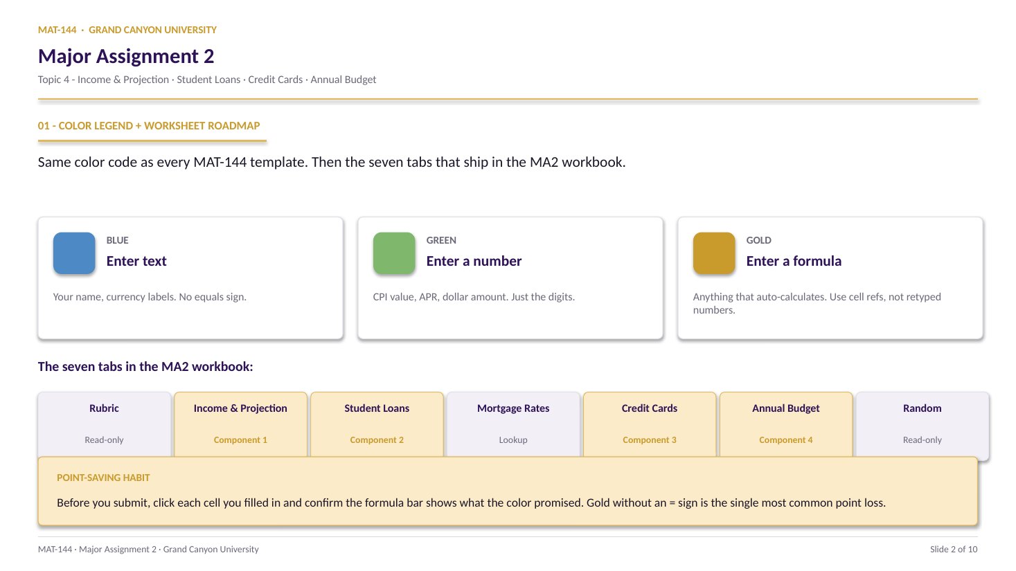
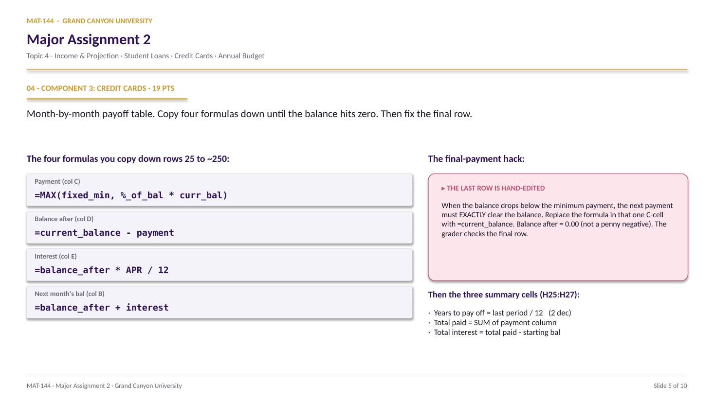
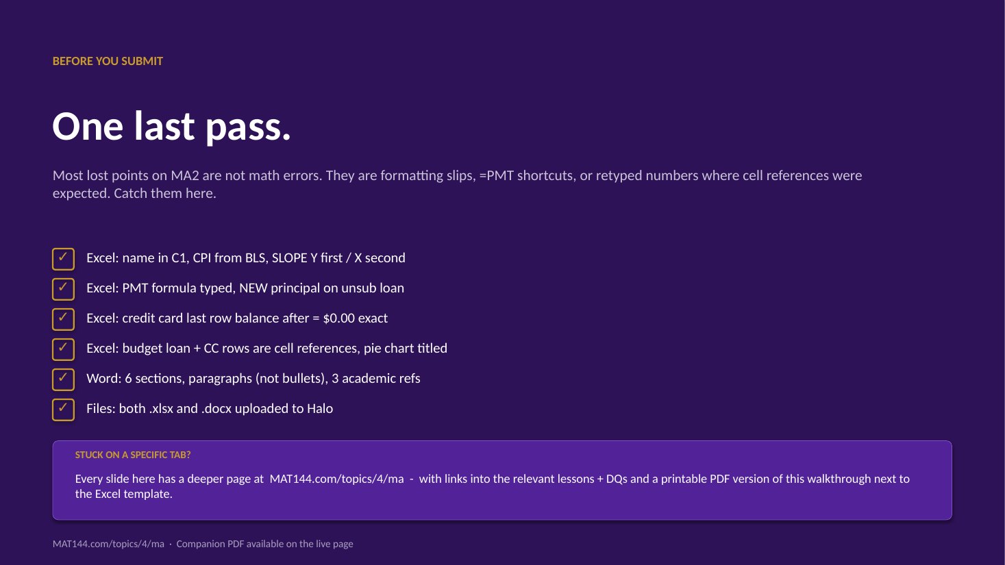
TOPIC 4 · MAJOR ASSIGNMENT 2 · COMPONENT 02/ Financial Literacy / major assignment / student loans
02Two loans, one ten-year clock.
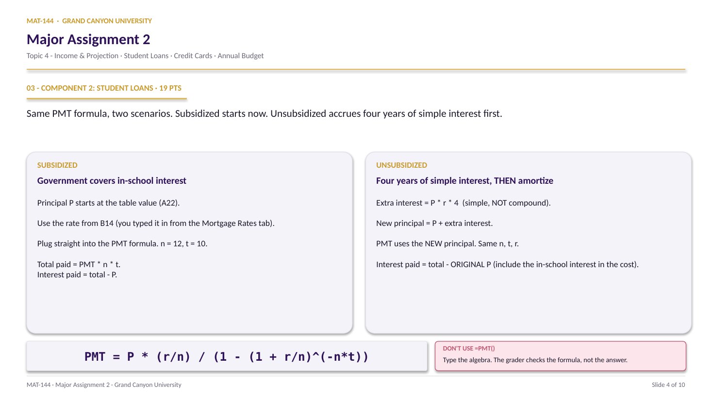
Look up a historical APR from the Mortgage Rates tab. Type the PMT formula out by hand (no =PMT shortcut). Run it on the subsidized principal AND on the unsubsidized principal grown by four years of simple interest. Compare what you actually pay.
Major Assignment · 19% of Excel
n = 12 · t = 10
Algebra, not =PMT()
A 7-page MA2 Walkthrough PDF covers all four components in the same hint depth as this page. Useful if you'd rather print, annotate on paper, or keep it open on a second screen while working in Excel.
Walkthrough video coming in a future recording. Until then, work from the slideshow above and the printable PDF.
SCRIBE.HOW · YOUTUBE
≡
Step-by-step walkthrough
Coming soon. Check back after the Scribe is recorded.
▸
Video walkthrough
Coming soon. Work from the slideshow and printable PDF until then.
The Topic 4 Review Q4 video walks the same subsidized-vs-unsubsidized computation MA2 C2 asks you to run on your own loan numbers. The move: subsidized keeps Prepay = original P, while unsubsidized grows P first by P·r·tschool (simple interest during school), then runs the amortization formula. Same math, worked on video — swap the numbers in as you go.
Same walkthrough, three modes.Pick the one that lands for you today.
ORIENT
· the tab
APR first, then two parallel columns.
Lookup keys auto-populate. You type the APR. Then run subsidized math on the left, unsubsidized math on the right. Same formula, two different principals.
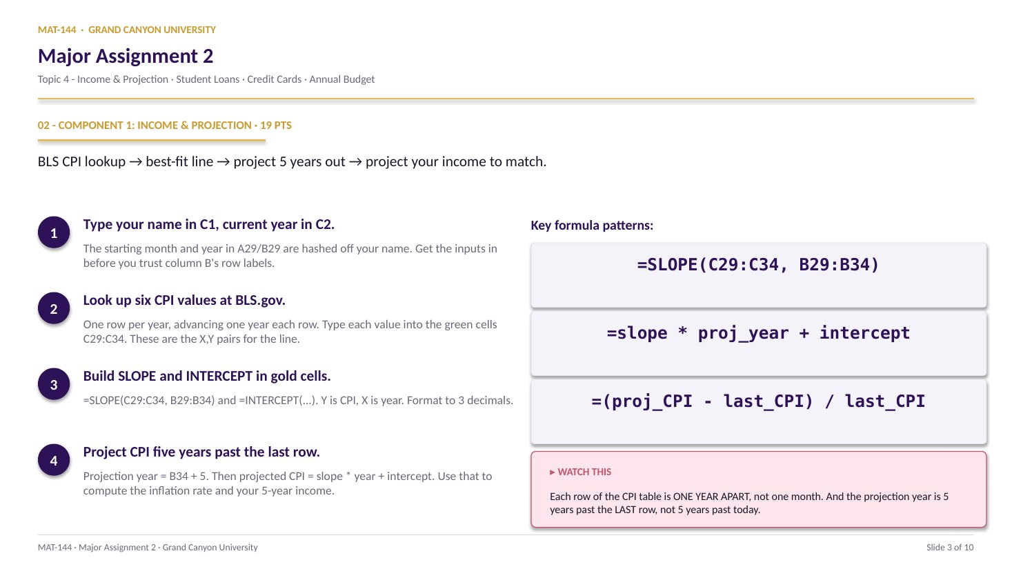
Cells B12 and B13 auto-generate your personalized year and month - your lookup key into the Mortgage Rates tab. Cross-reference there, type the APR you find into green cell B14, and the loan principal in A22 spawns from your name hash. From there it’s two parallel columns of arithmetic.
§1 · Lookup
Mortgage Rates tab → B14.
B12 = year, B13 = month. Both auto-populated. Open the Mortgage Rates tab, find the cell at that (row, column) intersection, copy the APR into B14. Format as Percentage with 2 decimals.
Type the PMT formula out by hand with cell references for P (A22), r (B14), n (12), t (10). Total paid = PMT × n × t. Interest paid = total - P.
§3 · Unsubsidized
E25 accrual, E26 new P, E29-E31 totals.
E25 = P · r · 4 (four years of simple interest, in-school). E26 = P + accrual. Then run the same PMT formula on the grown principal. Interest paid subtracts the original A22, not the grown principal.
CONCEPTS · six things to know
The four moves of both columns.
PMT is the same formula either way. The only thing that changes is what you feed in as P. Get that right and the rest is arithmetic.
01
Lookup
B12 + B13 point you at the APR.
Open the Mortgage Rates tab. It’s a 1971-present table with years down the left and months across the top. Match the year in B12 to a row, the month in B13 to a column, and read the APR at the intersection.
Type that APR into green cell B14 on the Student Loans tab. Format as Percentage with 2 decimals. Every formula on the rest of the tab references B14 - so if you get this wrong, every downstream number is wrong too.
A
B
C
7
label
a
b
8
12
7
9
sum
=B8+C8
19
change B8→ C9 follows
02
PMT
Type the algebra. No =PMT().
The formula in plain Excel is =A22*(B14/12)/(1-(1+B14/12)^(-12*10)). P from A22 (your principal), r from B14 (your APR), n = 12, t = 10. Type it literally; don’t shortcut.
The grader checks the formula bar, not just the answer. =PMT(B14/12,120,-A22) returns the right number but reads as zero-credit. The point of the assignment is can you write down the formula yourself.
=P*(r/n) / (1 - (1+r/n)^(-n*t))
P = A22 · r = B14 · n = 12 · t = 10
All cell references. No typed numbers anywhere.
03
Total + interest
PMT × n × t, then total - P.
Total paid in B30: =B29 * 12 * 10. That’s 120 monthly payments over 10 years - the lifetime cash flow out of your pocket.
Interest paid in B31: =B30 - A22. Total cash out, minus the principal you borrowed, equals the interest the lender kept. Format both as Currency.
=SUM(E21:E28)
=Switch on
SUMFunction name
( )Argument hold
E21:E28Range arg
04
Simple
Unsubsidized accrual: I = P · r · 4.
Four years of in-school accrual on the unsubsidized loan. Cell E25: =A22 * B14 * 4. Simple interest, not compound - the interest grows linearly. New principal at graduation goes in E26: =A22 + E25.
From E26 onward, the unsubsidized math runs the same PMT formula as subsidized - just with the grown principal instead of A22. Everything downstream cell-references E26.
E25 = A22 * B14 * 4
Linear growth. Four years of interest only.
E26 = A22 + E25 then feeds the PMT formula.
05
Subtract
Unsubsidized interest paid = total - original P.
The trap: E31 wants =E30 - A22, not =E30 - E26. Subtract the original principal so the in-school interest counts as interest paid.
If you subtract E26 (the grown principal), you’ll hide the in-school accrual and the unsubsidized loan will look artificially cheap. That defeats the entire point of the side-by-side comparison.
Stored in cell
1.1428571428571428
Displayed (2 dec.)
1.14
Common slips
Four mistakes that cost the most points.
The =PMT() shortcut and the simple-vs-compound confusion are the two big point-killers. Read your formula bar before you submit.
01
Used =PMT().
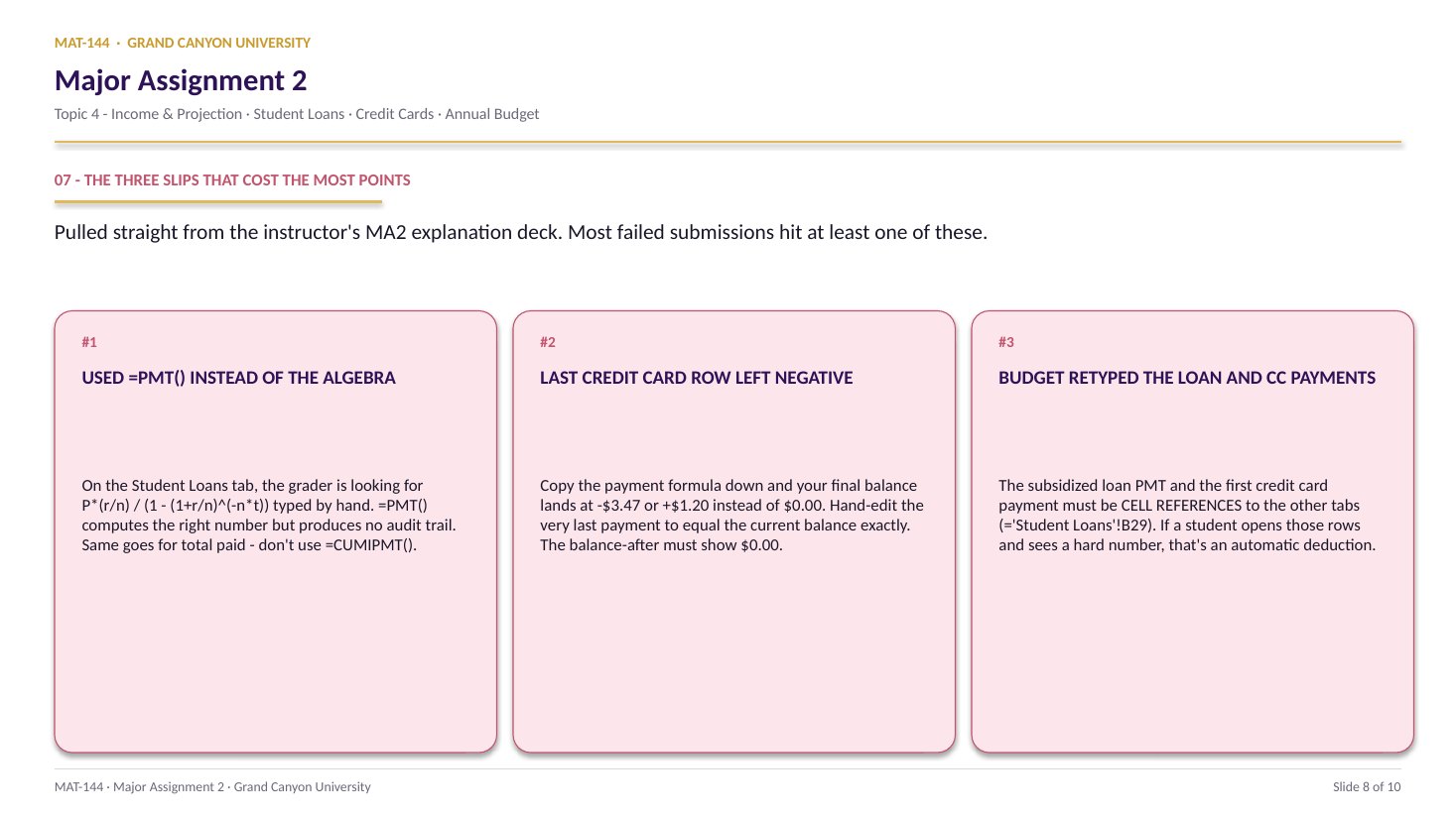
The Excel built-in returns the right number but is explicitly forbidden. Type the algebra: =A22*(B14/12)/(1-(1+B14/12)^(-120)). The grader audits the formula bar.
02
Compounded the in-school interest.
Four years of in-school accrual on the unsubsidized loan is simple interest (=P*r*4), not compound. If your accrual is bigger than ~4r · P, you compounded. Simple interest grows linearly - one r per year, added.
03
Subtracted the grown principal, not the original.
Unsubsidized interest paid is =total - A22, not =total - E26. Subtract the original principal so the in-school interest counts as interest paid.
04
Dropped the /n in the PMT formula.
The periodic rate is r/n, not r. If your monthly payment looks like a yearly payment (way too big), you wrote (1+r)^(-n*t) instead of (1+r/n)^(-n*t). Add the /12 back in everywhere r appears.
Application & connection
This is DQ 2 plus simple interest, in tab form.
This component is Topic 4 DQ 2 dressed up for prime time. The PMT formula is identical. The simple-interest accrual on the unsubsidized loan is Lesson 5 unchanged - I = P · r · t, with t = 4. Two formulas, two columns, one ten-year clock.
The reason the assignment forbids =PMT() isn’t pedantry. It’s that when you write the formula out, you can see what each piece does: P*r/n is the interest portion of the first payment; the denominator is the geometric-series adjustment that spreads the loan across n · t periods. =PMT() hides all of that. Typing the algebra puts it back.
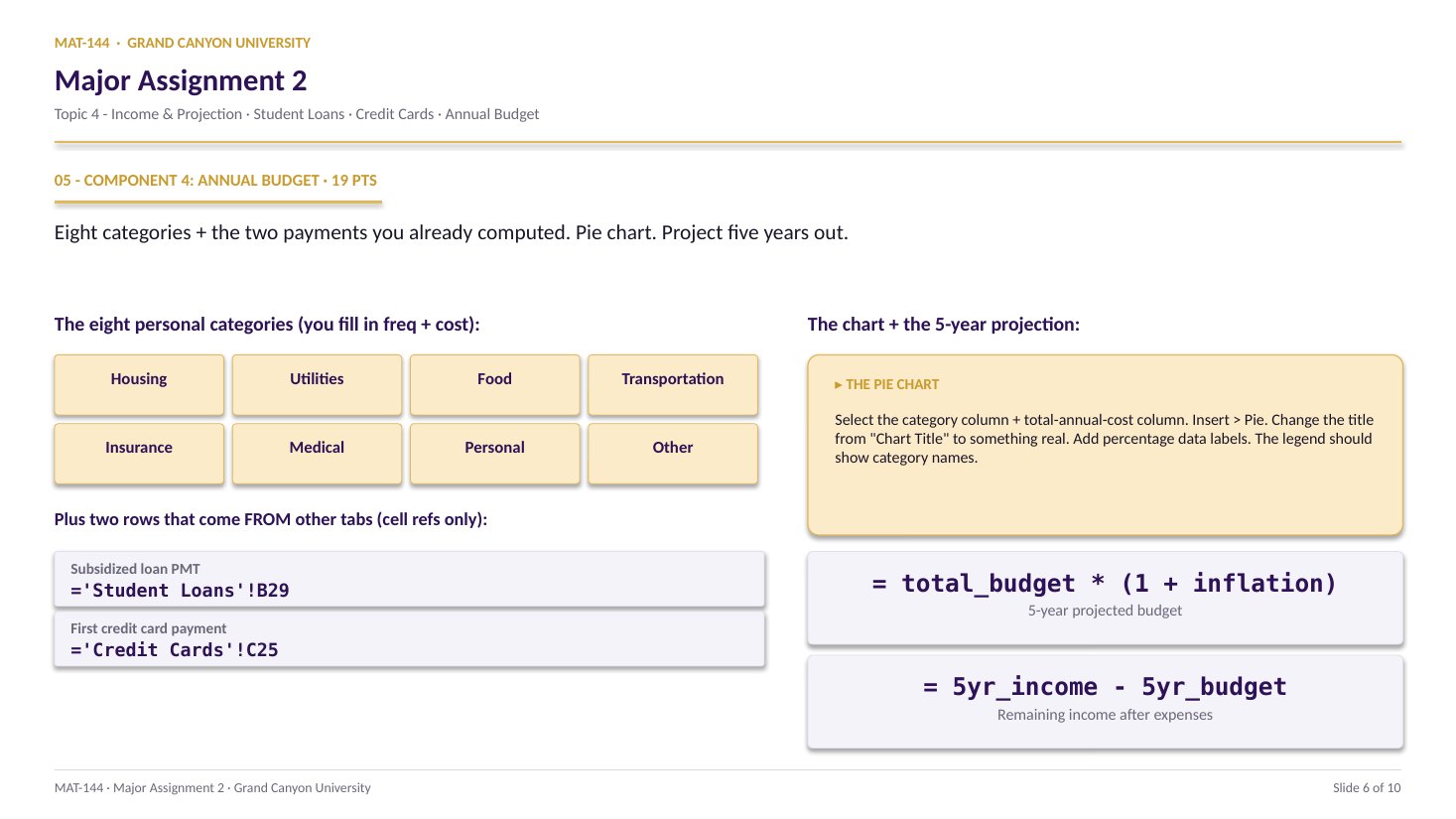
The subsidized PMT carries forward into the Annual Budget tab (Component 4) - the loan-payment line there is a cell reference to B29, not a retyped number.