TOPIC 3 · DQ 1 / Savings / discussion question

01Plug the formulas in. Watch them work.

Four problems on the Financial tab walk you through every future-value formula in this topic — simple, compound, annuity, and the reverse "how much do I save each month?" calculation.

Discussion · 5 pts Initial post Wed · replies Sun Future value Annuity FV

▸ The why · 7-slide reference

1 / 7

↓ Download .pptx

Step 1 · materials

Download the worksheet

Topic_3_DQ_1.xlsx

XLSX 5 pts v · spring 26

Step 2 · walkthrough

Watch the click-by-click

Every keystroke for all four problems. The Scribe walkthrough lands here once recorded; for now, the Excel template above is your working surface.

SCRIBE.HOW · YOUTUBE

Step-by-step walkthrough

Coming soon. Check back after the Scribe is recorded.

Same walkthrough, two modes. Use whichever helps you today.

Open the Financial tab. Type your name in the blue cell at the top — the inputs (P, r, t) for the four problems are generated from your name, so your version is unique. The four problems map directly to the topic's four future-value formulas. Self-check colors tell you whether each answer cell got the right value and whether you used a formula to get there. Both have to be green for credit. New to the cell color codes? See the legend.

§1 · Simple interest

FV = P(1 + rt).

One-time deposit, no compounding. Lesson 2's formula, in spreadsheet form.

§2 · Compound interest

FV = P(1 + r/n)^(nt).

Same deposit, now compounded n times per year. Lesson 3's formula.

§3 · Annuity (forward)

FV = P((1+r/n)^(nt) − 1)/(r/n).

Stream of monthly deposits of P each. Lesson 5's annuity FV formula.

§4 · Solve for M

P = FV(r/n)/((1+r/n)^(nt) − 1).

Reverse direction: how much do I save each month to reach a target FV? The most useful formula in personal finance.

Problem 1 · Simple

Simple interest, cell-reference style.

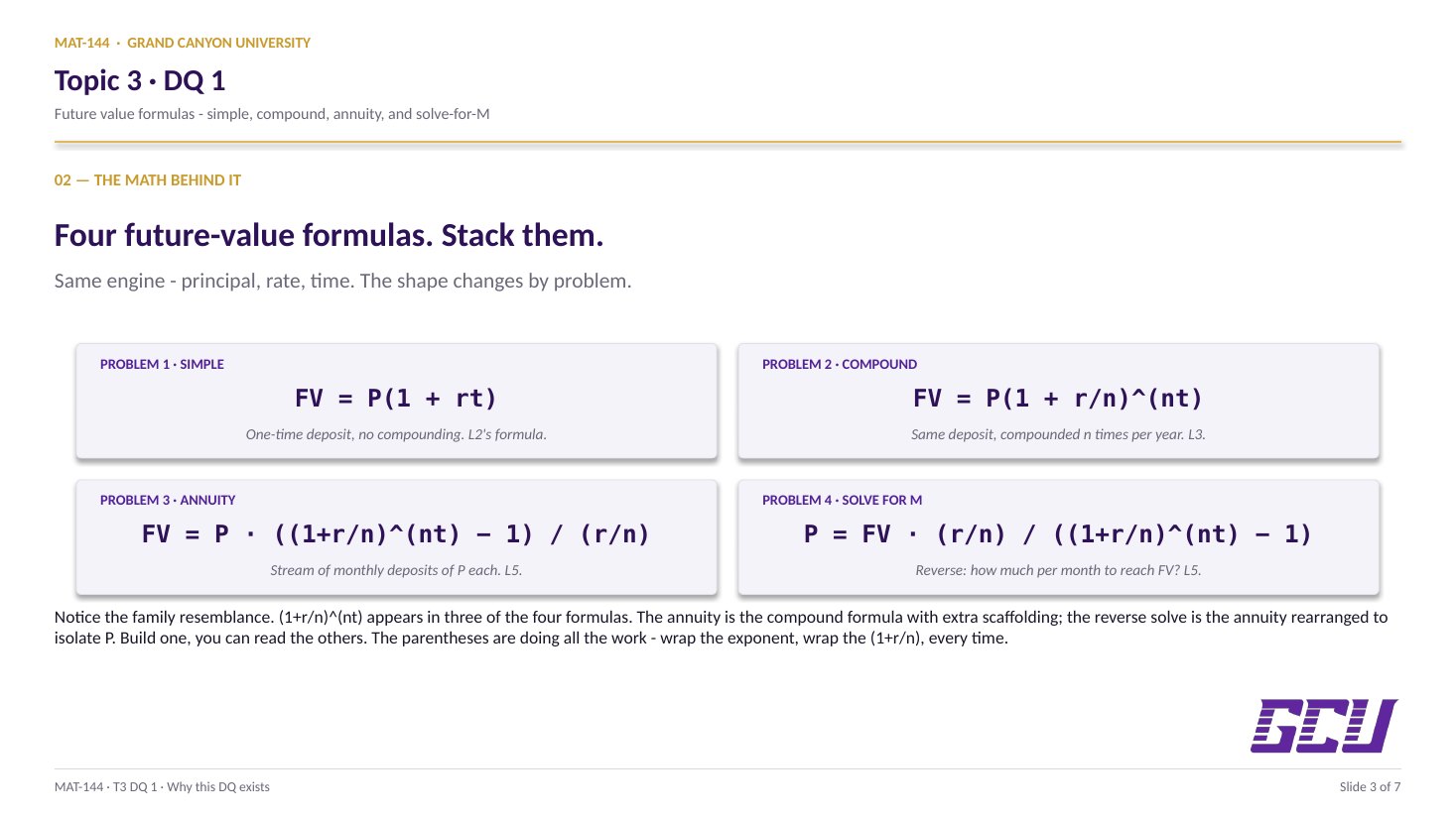
Problem 1: Simple interest, one-time deposit. You're given P, r, n=12 (always monthly compounding for these problems), and t. You compute the future value FV using the simple-interest formula, then the interest earned (FV − P).

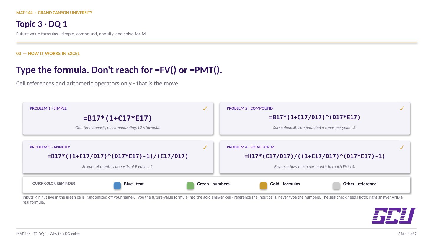
The Excel formula goes into the gold cell: =B20*(1+C20*E20) — where B20 is your randomized P, C20 is your randomized r (already as a decimal), and E20 is t. Note that n doesn't appear; simple interest doesn't compound.

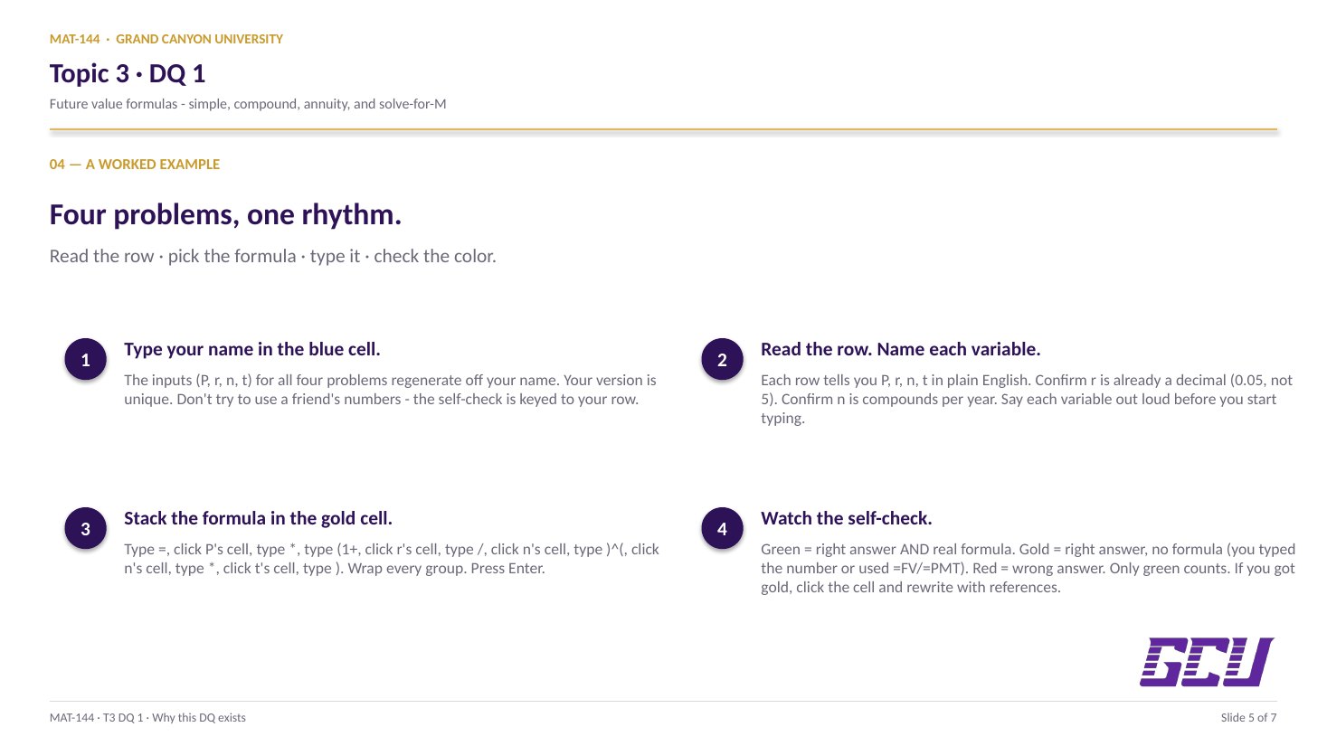
Interest earned: subtract P from FV. =H17-B20 in the gold cell next to it. The sheet checks that you used a subtraction formula, not the typed difference.

This is the same recipe from Lesson 2, just with cell references replacing the numbers.

Problem 2 · Compound

Compound interest, parens matter.

Problem 2: Compound interest, one-time deposit. Same P, r, n, t — but now the formula is FV = P(1 + r/n)^nt. The compounding frequency n now matters: with n=12, interest compounds monthly during the time period.

The Excel formula: =B24*(1+C24/D24)^(D24*E24). Watch every parenthesis. The exponent D24*E24 needs to be in parentheses because Excel evaluates ^ right-to-left and treats ^a*b very differently from ^(a*b).

Interest earned: same idea — =H21-B24.

Sanity check against simple: with the same inputs, compound should give a slightly larger FV. If your simple answer is bigger than your compound answer, a parenthesis is in the wrong place.

Problem 3 · Annuity

A stream of deposits, compounded.

Problem 3: Annuity FV (periodic deposits). Now P is a monthly deposit (not a starting principal). You're given the monthly amount, r, n=12, and t. The formula is the annuity future value from Lesson 5: FV = P · ((1 + r/n)^nt − 1) / (r/n).

The Excel formula: =B29*((1+C29/D29)^(D29*E29)-1)/(C29/D29). The big trap on this row is the dual use of (1+r/n)^(nt) − 1 inside one bracket — you have to subtract 1 before dividing by r/n. The structure: numerator is everything in the outer brackets minus 1; denominator is r/n.

This problem also asks for total invested (=B29*D29*E29 = P times n times t = monthly amount × 12 × years) and interest earned (FV − total invested). The interest-earned figure is usually surprisingly large — that's compounding doing the work over time.

Problem 4 · Reverse

The same formula rearranged for M.

Problem 4: Solve for M to reach a goal. The reverse direction. You're given a future-value goal (generated from your previous answer to Problem 2 or Problem 3), r, n, t. You compute the monthly payment that gets you there. The formula is the annuity formula solved for P:

P = FV · (r/n) / ((1 + r/n)^nt − 1)

The Excel formula: =B34*(C34/D34)/((1+C34/D34)^(D34*E34)-1). Notice the denominator is the same (1+r/n)^(nt) − 1 structure from Problem 3 — you're just rearranging the equation.

Then total invested (=H31*D34*E34) and interest earned (=B34-I31). Note interest in this case is FV − total invested, since the goal is the FV.

This is the most practical formula in the whole topic — it answers "how much do I need to save each month to hit $X by year Y?", which is the Topic 6 finale question made concrete.

Rule

Why =FV() and =PMT() are off-limits.

The DQ instructions are explicit: do not use the built-in =FV() and =PMT() functions. You have to type the formulas manually with cell references and arithmetic operators.

Two reasons. First: writing the formula yourself is the actual skill the DQ is testing. Excel's =FV() takes a different parameter order from the textbook formula, and it returns negative numbers for some sign conventions — using it without understanding it is a recipe for wrong-sign answers. Second: Major Assignment 2 in Topic 4 reuses the same formula shapes with a different scenario (loans). If you've typed FV = P(1+r/n)^(nt) by hand once, the loan amortization formula in MA2 is the same finger memory.

The self-check on the Financial tab catches this: if you plug in the right number directly without using a formula, the cell turns gold (right answer, no formula) instead of green (right answer, formula used). Gold means you got the answer but skipped the skill.

=FV(...)

built-in

rejected by this DQ
different param order
different sign convention

=B24*(1+C24/D24)^(D24*E24)

manual formula

required by this DQ
matches textbook
same shape used in MA2

Common slips

Five mistakes this DQ punishes.

Read these before you submit. The parenthesis slips on Problem 2 and Problem 3 are by far the most common.

01

Used =FV() or =PMT().

Explicitly off-limits for this DQ. The instructor catches it via the self-check; the cell turns gold (right number, no formula) instead of green. Type the formula manually with cell references and arithmetic operators.
02

Wrong parentheses on the exponent.

(1+r/n)^n*t means (1+r/n)ⁿ × t — totally different from (1+r/n)^n×t. Wrap the exponent: (1+r/n)^(n*t). Always.
03

Used the rate as 5 instead of 0.05.

The randomized r in the green cells is already a decimal (e.g. 0.05 for 5%). Don't multiply by 100 again. If your FV is wildly bigger than your principal, this is usually why.
04

Confused P (principal) with P (monthly payment).

Problem 1 and 2 use P as a one-time principal deposit. Problems 3 and 4 use P as a monthly periodic payment (or M). The formulas look similar; the meaning of P doesn't.
05

Subtracted 1 in the wrong place.

The annuity formula's structure is P × ((1+r/n)^(nt) − 1) / (r/n). The − 1 goes inside the outer brackets, not at the end. Misplace it and your answer is roughly wrong by a factor of (1+r/n)^(nt).

Application & connection

From this DQ into MA2.

This DQ exercises four formulas you already know: Lesson 2 (simple interest, FV = P(1+rt)), Lesson 3 (compound interest with frequency, FV = P(1+r/n)^nt), and Lesson 5 (annuity future value, both forward and reverse). The Excel template is your place to confirm: same recipe, different inputs, formula auto-updates if a value changes.

What I'm watching in your formulas: the parentheses around (1 + r/n), the exponent shape ^(n*t) not ^n*t, and that you wrote the formula yourself instead of leaning on Excel's built-in =FV() or =PMT(). Those are explicitly off-limits for this DQ — partly because building the formula by hand is the actual skill, and partly because Major Assignment 2 in Topic 4 (loans) uses the same formula shapes with new labels. Get fluent here, save time there.